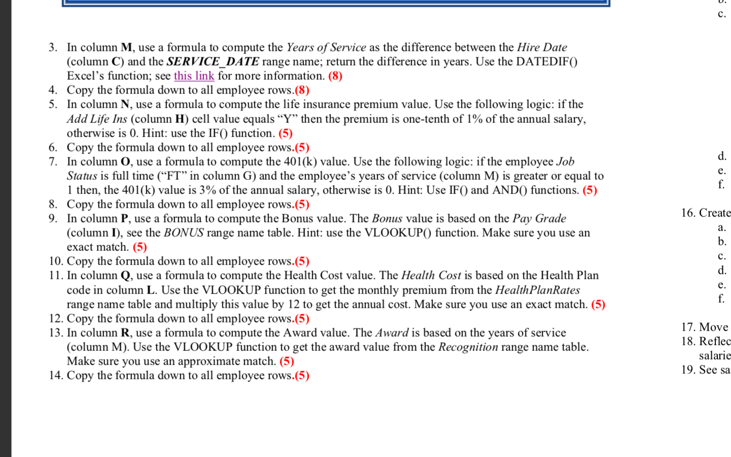
3. In column M, use a formula to compute the Years of Service as the difference between the Hire Date (column C) and the SERVICE_DATE range name; return the difference in years. Use the DATEDIF() Excel's function; see this link for more information. (8) 4. Copy the formula down to all employee rows.(8) 5. In column N, use a formula to compute the life insurance premium value. Use the following logic: if the Add Life Ins (column H ) cell value equals "Y" then the premium is one-tenth of 1% of the annual salary, otherwise is 0 . Hint: use the IF() function. (5) 6. Copy the formula down to all employee rows.(5) 7. In column O, use a formula to compute the 401(k) value. Use the following logic: if the employee Job Status is full time ("FT" in column G) and the employee's years of service (column M) is greater or equal to 1 then, the 401(k) value is 3% of the annual salary, otherwise is 0 . Hint: Use IF() and AND() functions. (5) 8. Copy the formula down to all employee rows.(5) 9. In column P, use a formula to compute the Bonus value. The Bonus value is based on the Pay Grade (column I), see the BONUS range name table. Hint: use the VLOOKUP() function. Make sure you use an exact match. (5) 10. Copy the formula down to all employee rows.(5) 11. In column Q, use a formula to compute the Health Cost value. The Health Cost is based on the Health Plan code in column L. Use the VLOOKUP function to get the monthly premium from the HealthPlanRates range name table and multiply this value by 12 to get the annual cost. Make sure you use an exact match. (5) 12. Copy the formula down to all employee rows.(5) 13. In column R, use a formula to compute the Award value. The Award is based on the years of service (column M). Use the VLOOKUP function to get the award value from the Recognition range name table. Make sure you use an approximate match. (5) 14. Copy the formula down to all employee rows.(5) 3. In column M, use a formula to compute the Years of Service as the difference between the Hire Date (column C) and the SERVICE_DATE range name; return the difference in years. Use the DATEDIF() Excel's function; see this link for more information. (8) 4. Copy the formula down to all employee rows.(8) 5. In column N, use a formula to compute the life insurance premium value. Use the following logic: if the Add Life Ins (column H ) cell value equals "Y" then the premium is one-tenth of 1% of the annual salary, otherwise is 0 . Hint: use the IF() function. (5) 6. Copy the formula down to all employee rows.(5) 7. In column O, use a formula to compute the 401(k) value. Use the following logic: if the employee Job Status is full time ("FT" in column G) and the employee's years of service (column M) is greater or equal to 1 then, the 401(k) value is 3% of the annual salary, otherwise is 0 . Hint: Use IF() and AND() functions. (5) 8. Copy the formula down to all employee rows.(5) 9. In column P, use a formula to compute the Bonus value. The Bonus value is based on the Pay Grade (column I), see the BONUS range name table. Hint: use the VLOOKUP() function. Make sure you use an exact match. (5) 10. Copy the formula down to all employee rows.(5) 11. In column Q, use a formula to compute the Health Cost value. The Health Cost is based on the Health Plan code in column L. Use the VLOOKUP function to get the monthly premium from the HealthPlanRates range name table and multiply this value by 12 to get the annual cost. Make sure you use an exact match. (5) 12. Copy the formula down to all employee rows.(5) 13. In column R, use a formula to compute the Award value. The Award is based on the years of service (column M). Use the VLOOKUP function to get the award value from the Recognition range name table. Make sure you use an approximate match. (5) 14. Copy the formula down to all employee rows