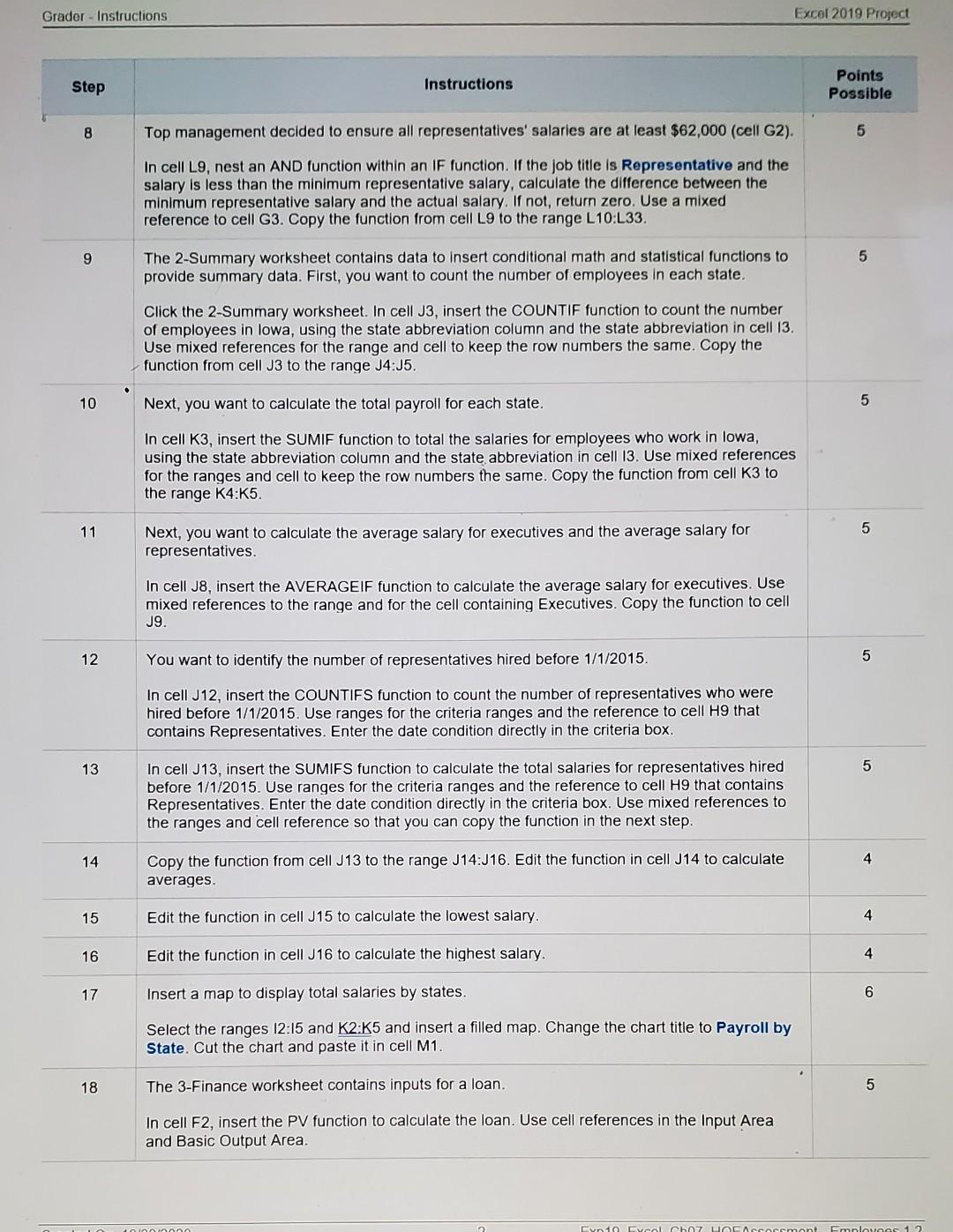
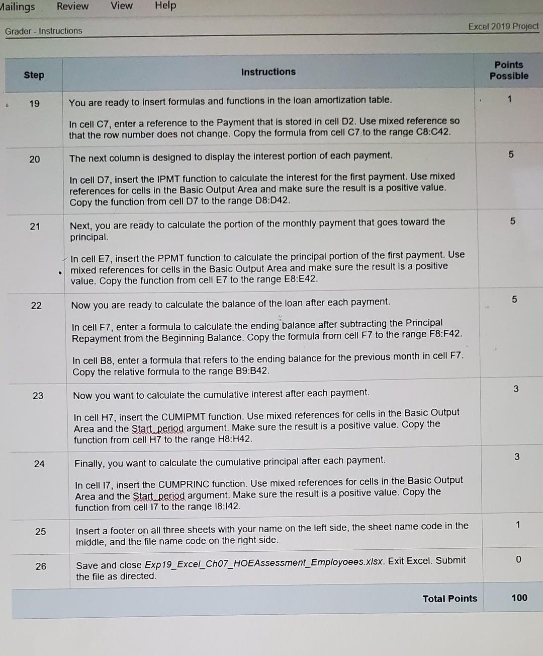
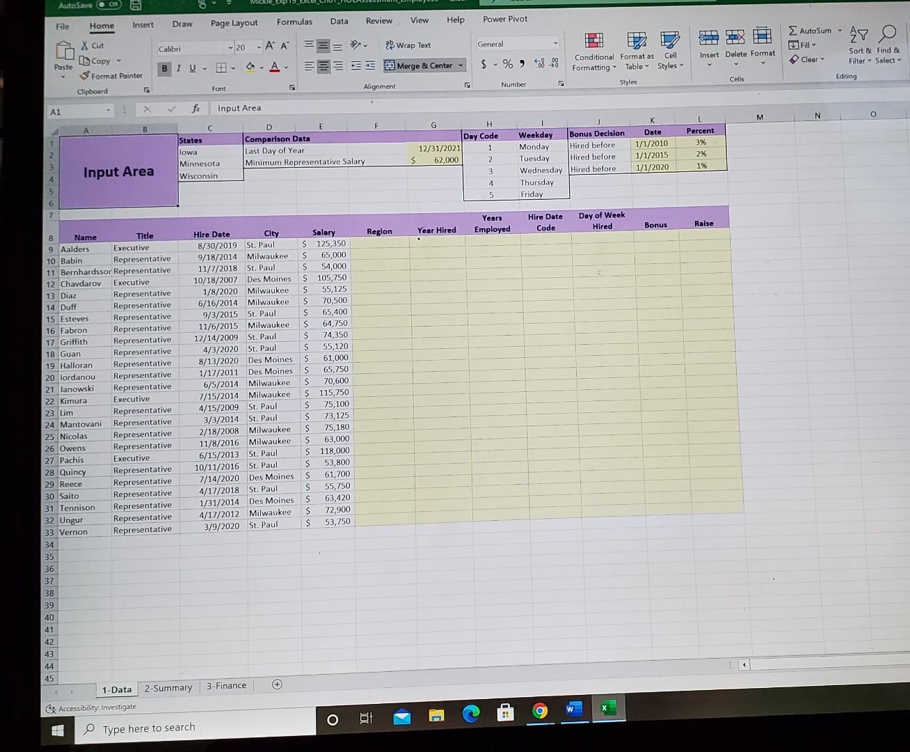
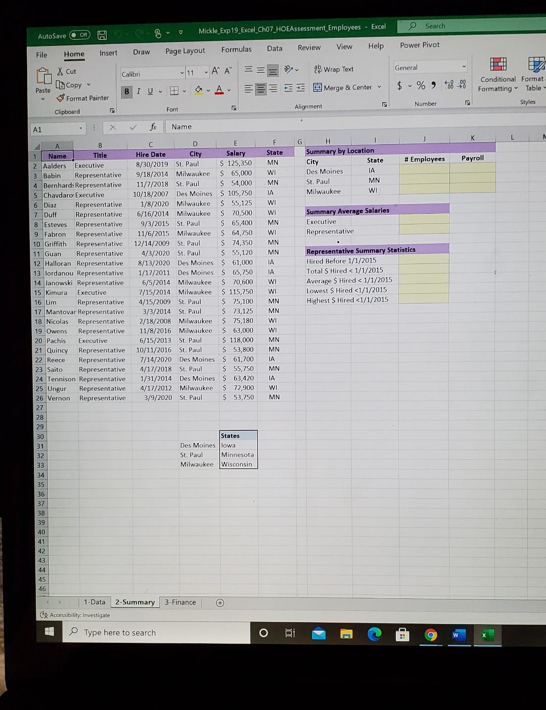
Grader - Instructions Excel 2019 Project Exp19_Excel_Ch07_HOEAssessment Employees Project Description: You work for a clothing distributor that has locations in lowa, Minnesota, and Wisconsin. You will use date and logical functions to complete the main employee data set, use database functions to calculate key summary statistics and create a map, and use financial functions to complete a loan amortization table. Steps to Perform: Step Instructions Points Possible 0 1 Start Excel. Download and open the file named Exp19_Excel_Cho7_HOEAssessment Employees.xlsx. Grader has automatically added your last name to the beginning of the filename. 3 2 The 1-Data worksheet contains employee data. You will insert several functions to complete this worksheet. Column C contains the actual hire dates for the employees. You want to extract only the year in column G. In cell G9, insert the appropriate date function to extract the year from the date in cell C9. Copy the function from cell G9 to the range G10:G33. 3 3 Next, you want to determine how many years each employee has worked for the company. In cell H9, insert the YEARFRAC function to calculate the years between the hire date and the last day of the year contained in cell G2. Use a mixed reference to cell G2. Copy the function from cell H9 to the range H10:H33. 4 4 You want to determine what day of the week each employee was hired. In cell 19, insert the WEEKDAY function to display the day of the week the first employee was hired. Use 2 as the return type. Copy the function from cell 19 to the range 110:133. 5 5 The value returned in cell 19 is a whole number. You want to display the weekday equivalent. In cell J9, insert a VLOOKUP function to look up the value stored in cell 19, compare it to the array in the range H2:16, and return the day of the week. Use mixed references to the table array. Copy the function from cell J9 to the range J10:J33. 4 6 Column D contains the city each employee works in. You want to display the state. In cell F9, insert the SWITCH function to switch the city stored in cell D9 with the respective state contained in the range C2:C4. Switch Des Moines for lowa, St. Paul for Minnesota, and Milwaukee for Wisconsin. Use mixed references to cells C2, C3, and C4. Copy the function from cell F9 to the range F10:F33. 5 7 Your next task is to calculate the bonus for the first employee. If the employee was hired before 1/1/2010, the employee's salary is multiplied by 3%. If the employee was hired before 1/1/2015, the employee's salary is multiplied by 2%. If the employee was hired before 1/1/2020, the employee's salary is multiplied by 1%. In cell K9, insert the IFS function to create the three logical tests to calculate the appropriate bonus. Use mixed references to cells within the range K2:L4. Copy the function from cell K9 to the range K10:K33. O W C Grader - Instructions Excel 2019 Project Step Instructions Points Possible 8 Top management decided to ensure all representatives' salaries are at least $62,000 (cell G2). 5 In cell L9, nest an AND function within an IF function. If the job title is Representative and the salary is less than the minimum representative salary, calculate the difference between the minimum representative salary and the actual salary. If not, return zero. Use a mixed reference to cell G3. Copy the function from cell L9 to the range L10:L33. 9 5 The 2-Summary worksheet contains data to insert conditional math and statistical functions to provide summary data. First, you want to count the number of employees in each state. Click the 2-Summary worksheet. In cell J3, insert the COUNTIF function to count the number of employees in Iowa, using the state abbreviation column and the state abbreviation in cell 13. Use mixed references for the range and cell to keep the row numbers the same. Copy the function from cell J3 to the range J4:J5. 10 Next, you want to calculate the total payroll for each state. 5 In cell K3, insert the SUMIF function to total the salaries for employees who work in lowa, using the state abbreviation column and the state abbreviation in cell 13. Use mixed references for the ranges and cell to keep the row numbers the same. Copy the function from cell K3 to the range K4:55. 11 5 Next, you want to calculate the average salary for executives and the average salary for representatives In cell J8, insert the AVERAGEIF function to calculate the average salary for executives. Use mixed references to the range and for the cell containing Executives. Copy the function to cell J9. 12 You want to identify the number of representatives hired before 1/1/2015 5 In cell J12, insert the COUNTIFS function to count the number of representatives who were hired before 1/1/2015. Use ranges for the criteria ranges and the reference to cell H9 that contains Representatives. Enter the date condition directly in the criteria box. 13 5 In cell J13, insert the SUMIFS function to calculate the total salaries for representatives hired before 1/1/2015. Use ranges for the criteria ranges and the reference to cell H9 that contains Representatives. Enter the date condition directly in the criteria box. Use mixed references to the ranges and cell reference so that you can copy the function in the next step. 14 4 Copy the function from cell J13 to the range J14:J16. Edit the function in cell J14 to calculate averages. 15 Edit the function in cell J15 to calculate the lowest salary. 4 16 Edit the function in cell J16 to calculate the highest salary. 4 17 Insert a map to display total salaries by states. 6 Select the ranges 12:15 and K2:K5 and insert a filled map. Change the chart title to Payroll by State. Cut the chart and paste it in cell M1. 18 The 3-Finance worksheet contains inputs for a loan. 5 In cell F2, insert the PV function to calculate the loan. Use cell references in the Input Area and Basic Output Area. Yan Nycol Ch07 molous 1 2 Mailings Review View Help Excel 2019 Project Grader - Instructions Step Instructions Points Possible 1 19 You are ready to insert formulas and functions in the loan amortization table. In cell C7, enter a reference to the Payment that is stored in cell D2. Use mixed reference so that the row number does not change. Copy the formula from cell C7 to the range C8:C42. 5 20 The next column is designed to display the interest portion of each payment. In cell 07, insert the IPMT function to calculate the interest for the first payment. Use mixed references for cells in the Basic Output Area and make sure the result is a positive value. Copy the function from cell D7 to the range D8:D42. 5 21 Next, you are ready to calculate the portion of the monthly payment that goes toward the principal In cell E7, insert the PPMT function to calculate the principal portion of the first payment. Use mixed references for cells in the Basic Output Area and make sure the result is a positive value. Copy the function from cell E7 to the range E8:E42. 5 22 Now you are ready to calculate the balance of the loan after each payment. In cell F7, enter a formula to calculate the ending balance after subtracting the Principal Repayment from the Beginning Balance. Copy the formula from cell F7 to the range F8:F42. In cell B8, enter a formula that refers to the ending balance for the previous month in cell F7. Copy the relative formula to the range B9:B42. 3 23 Now you want to calculate the cumulative interest after each payment. In cell H7, insert the CUMIPMT function. Use mixed references for cells in the Basic Output Area and the start period argument. Make sure the result is a positive value. Copy the fun from cell H7 to the range H8:H42. 3 24 Finally, you want to calculate the cumulative principal after each payment. In cell 17, insert the CUMPRINC function. Use mixed references for cells in the Basic Output Area and the Start period argument. Make sure the result is a positive value. Copy the function from cell 17 to the range 18:142. 1 25 Insert a footer on all three sheets with your name on the left side, the sheet name code in the middle, and the file name code on the right side. 0 26 Save and close Exp19_Excel_Cho7_HOEAssessment_Employoees.xlsx. Exit Excel. Submit the file as directed. Total Points 100 AutoSave OOR Power Pivot TT TX ODO TH AutoSum Fill 28 O General Insert Delete Format Clear Sort By Find & Filter Select File Home Insert Draw Page Layout Formulas Data Review View Help X Cut Calibri - 20 - AA Wrap Text [Copy - Paste BI VE - ASSE Merge & Center Format Painter Font Alignment Clipboard A1 fi Input Area $ % 948_08 Conditional Format as Cell Formatting Table Styles Styles Cells Editing Number 5 M N o 1 C B F A States lowa Minnesota Wisconsin D E Comparison Data Last Day of Year Minimum Representative Salary G H Day Code 12/31/2021 1 S 62,000 2 3 Weekday Bonus Decision Monday Hired before Tuesday Hired before Wednesday Hired before Thursday Friday Date 1/1/2010 1/1/2015 1/1/2020 Percent 3% 2% 1% Input Area 4 5 7 Years Employed Hire Date Code Day of Week Hired Bonus Raise Region Year Hired 8 Name Title 9 Aalders Executive 10 Babin Representative 11 Bernhardssor Representative 12 Chavdarov Executive 13 Diaz Representative 14 Duff Representative 15 Esteves Representative 16 Fabron Representative 17 Griffith Representative 18 Guan Representative 19 Halloran Representative 20 lordanou Representative 21 Janowski Representative 22 Kimura Executive 23 Lim Representative 24 Mantovani Representative 25 Nicolas Representative 26 Owens Representative 27 Pachis Executive 28 Quincy Representative 29 Reece Representative 30 Saito Representative 31 Tennison Representative 32 Ungur Representative 33 Vernon Representative 34 35 Hire Date City 8/30/2019 St. Paul 9/18/2014 Milwaukee 11/1/2018 St. Paul 10/18/2007 Des Moines 1/8/2020 Milwaukee 6/16/2014 Milwaukee 9/3/2015 St. Paul 11/6/2015 Milwaukee 12/14/2009 St. Paul 4/3/2020 St. Paul 8/13/2020 Des Moines 1/17/2011 Des Moines 6/5/2014 Milwaukee 7/15/2014 Milwaukee 4/15/2009 St. Paul 3/3/2014 St. Paul 2/18/2008 Milwaukee 11/8/2016 Milwaukee 6/15/2013 St. Paul 10/11/2016 St. Paul 7/14/2020 Des Moines 4/17/2018 St. Paul 1/31/2014 Des Moines 4/17/2012 Milwaukee 3/9/2020 St. Paul Salary $ 125,350 $ 65,000 S 54,000 $ 105,750 S 55,125 S 70,500 $ 65,400 S 64,750 S 74,350 S 55,120 S 61,000 S 65,750 $ 70,600 $ 115,750 S 75,100 S 73,125 $ S 63,000 $ 118,000 S 53,800 S 61,700 S 55,750 S 63,420 S 72,900 $ 53,750 75,180 36 37 38 39 40 41 42 43 44 45 1-Data + 2-Summary 3- Finance y Accessibility: Investigate W o E Type here to search Search Mickle_Exp19_Excel_Cho7_HOEAssessment Employees - Excel AutoSave On Data Review Formulas View Help Power Pivot File Home Insert Draw Page Layout a Wrap Text General Calibri X Cut Ub Copy Format Painter 11 A A A- Paste $ % 9 408.08 BIU Es Merge & Center Conditional Format Formatting Table - Styles Number Font Alignment Clipboard X fx A1 Name L N G # Employees Payroll H Summary by Location City State Des Moines IA St. Paul MN Milwaukee WI Summary Average Salaries Executive Representative B 1 Name Title 2 Aalders Executive 3 Babin Representative 4 Bernhard: Representative 5 Chavdaro Executive 6 Diaz Representative 7 Duff Representative 8 Esteves Representative 9 Fabron Representative 10 Griffith Representative 11 Guan Representative 12 Halloran Representative 13 Iordanou Representative 14 Janowski Representative 15 Kimura Executive 16 Lim Representative 17 Mantovar Representative 18 Nicolas Representative 19 Owens Representative 20 Pachis Executive 21 Quincy Representative 22 Reece Representative 23 Saito Representative 24 Tennison Representative 25 Ungur Representative 26 Vernon Representative 27 D E Hire Date City Salary 8/30/2019 St. Paul $ 125,350 9/18/2014 Milwaukee $ 65,000 11/7/2018 St. Paul $ 54,000 10/18/2007 Des Moines $ 105,750 1/8/2020 Milwaukee $ 55,125 6/16/2014 Milwaukee $ 70,500 9/3/2015 St. Paul $ 65,400 11/6/2015 Milwaukee $ 64,750 12/14/2009 St. Paul $ 74,350 4/3/2020 St. Paul $ 55,120 8/13/2020 Des Moines $ 61,000 1/17/2011 Des Moines $ 65,750 6/5/2014 Milwaukee $ 70,600 7/15/2014 Milwaukee $ 115,750 4/15/2009 St. Paul $ 75,100 3/3/2014 St. Paul $ 73,125 2/18/2008 Milwaukee $ 75,180 11/8/2016 Milwaukee $ 63,000 6/15/2013 St. Paul $ 118,000 10/11/2016 St. Paul $ 53,800 7/14/2020 Des Moines $ 61,700 4/17/2018 St. Paul $ 55,750 1/31/2014 Des Moines $ 63,420 4/17/2012 Milwaukee $ 72,900 3/9/2020 St. Paul $ 53,750 F State MN WI MN IA WI WI MN WI MN MN IA IA WI WI MN MN WI WI MN MN IA MN IA WI MN Representative Summary Statistics Hired Before 1/1/2015 Total $ Hired 1-Data 2-Summary 3-Finance Cx Accessibility. Investigate Type here to search la Format Painter Merge & Center 000 Formatting Table Styles Styles Clipboard Font Alignment Number Cell F2 fx B F H L M A 1 Input Area: 2 Years 3 Pmts per Year 4 $ 3 12 Payment APR D E Basic Output Area: 750.00 Loan 4.75% Periodic Rate # of Payments 0.396% 36 5 Monthly Payment Beginning Balance $ Principal Repayment Ending Balance Cumulative Interest Cumulative Principal 6 Payment Number 1 2 Interest Paid 7 8 9 3 10 4 5 6 7 8 11 12 13 14 15 16 17 18 9 10 11 12 19 13 14 20 21 15 22 16 17 23 24 18 19 25 26 20 27 21 28 22 29 30 23 24 31 32 33 34 35 36 37 38 39 25 26 27 28 29 30 31 32 33 34 40 1-Data 2-Summary 3- Finance 0 f. Accessibility Investigate