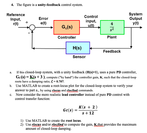
4. The figure is a unity-feedback control system. System Output y (t) Reference Error e(t) Control input, Input, r(t)+ 4 Gc(s) Controller Plant H(s) Feedback Sensor If this closed-loop system, with a unity feedback (H(s)-1), uses a pure PD controller Gc(s)-K(s +3), compute ("by hand") the controller gain, K, such that the closed-loop roots have a damping ratio, -0.707 Use MATLAB to create a root-locus plot for the closed-loop system to verify your answer to part a., by using rlocus and rlocfind commands. Now consider the more realistic lead controller instead of pure PD control with control transfer function: a. b. c. Gc(s) - K* + 2) s + 12 1) Use MATLAB to create the root locus. 2) Use rlocus and/or riocfind to compute the gain, K-that provides the maximum amount of closed-loop damping. 4. The figure is a unity-feedback control system. System Output y (t) Reference Error e(t) Control input, Input, r(t)+ 4 Gc(s) Controller Plant H(s) Feedback Sensor If this closed-loop system, with a unity feedback (H(s)-1), uses a pure PD controller Gc(s)-K(s +3), compute ("by hand") the controller gain, K, such that the closed-loop roots have a damping ratio, -0.707 Use MATLAB to create a root-locus plot for the closed-loop system to verify your answer to part a., by using rlocus and rlocfind commands. Now consider the more realistic lead controller instead of pure PD control with control transfer function: a. b. c. Gc(s) - K* + 2) s + 12 1) Use MATLAB to create the root locus. 2) Use rlocus and/or riocfind to compute the gain, K-that provides the maximum amount of closed-loop damping