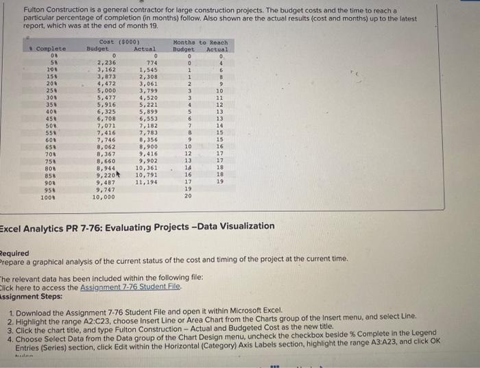
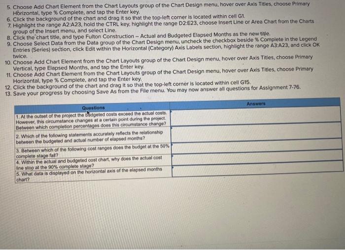
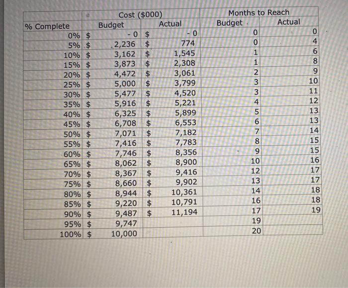
5. Choose Add Chart Element from the Chart Layouts group of the Chart Design menu, hover over Axis Titles, choose Primary Horizontal, type \% Complete, and tap the Enter key. 6. Click the background of the chart and drag it so that the top-left corner is located within cell G1. 7. Highlight the range A2:A23, hold the CTRL key, highlight the range D2:E23, choose Insert Line or Area Chart from the Charts group of the Insert menu, and select Line. 8. Click the chart title, and type Fulton Construction - Actual and Budgeted Elapsed Months as the new title. 9. Choose Select Data from the Data group of the Chart Design menu, uncheck the checkbox beside \% Complete in the Legend Entries (Series) section, click Edit within the Horizontal (Category) Axis Labels section, highlight the range A3:A23, and click OK twice. 10. Choose Add Chart Element from the Chart Layouts group of the Chart Design menu, hover over Axis Titles, choose Primary Vertical, type Elapsed Months, and tap the Enter key. 11. Choose Add Chart Element from the Chart Layouts group of the Chart Design menu, hover over Axis Titles, choose Primary Horizontal, type \% Complete, and tap the Enter key. 12. Click the background of the chart and drag it so that the top-left corner is located within cell G15. 13. Save your progress by choosing Save As from the Flle menu. You may now answer all questions for Assignment 7-76. Fulton Construction is a general contractor for large construction projects. The budget costs and the time to reach a particular percentage of completion (in months) follow. Also shown are the actual results (cost and months) up to the latest report, which was at the end of month 19. Excel Analytics PR 7-76: Evaluating Projects -Data Visualization Pequired repare a graphical analysis of the current status of the cost and timing of the project at the current time. he relevant data has been included within the following file: lick here to access the Assignment 7-76 Student File. ssignment Steps: 1. Download the Assignment 7-76 Student File and open it within Microsoft Excel. 2. Highlight the range A2:C23, choose Insert Line or Area Chart from the Charts group of the Insert menu, and select Line. 3. Click the chart title, and type Fulton Construction - Actual and Budgeted Cost as the new title. 4. Choose Select Data from the Data group of the Chart Design menu, uncheck the checkbox beside \% Complete in the Legend Entries (Series) section, click Edit within the Horizontal (Category) Axis Labels section, highlight the range A3:A23, and click OK \begin{tabular}{|c|c|c|c|c|c|c|c|} \hline \multirow[b]{2}{*}{% Complete } & \multicolumn{4}{|c|}{ Cost ($000)} & \multicolumn{3}{|c|}{ Months to Reach } \\ \hline & & udget & & tual & Budget . & Actual & \\ \hline 0% & $ & -0 & $ & -0 & 0 & & 0 \\ \hline 5% & $ & 2,236 & $ & 774 & 0 & & 4 \\ \hline 10% & $ & 3,162 & $ & 1,545 & 1 & & 6 \\ \hline 15% & $ & 3,873 & $ & 2,308 & 1 & & 8 \\ \hline 20% & $ & 4,472 & $ & 3,061 & 2 & & 9 \\ \hline 25% & $ & 5,000 & $ & 3,799 & 3 & & 10 \\ \hline 30% & $ & 5,477 & $ & 4,520 & 3 & & 11 \\ \hline 35% & $ & 5,916 & $ & 5,221 & 4 & & 12 \\ \hline 40% & $ & 6,325 & $ & 5,899 & 5 & & 13 \\ \hline 45% & $ & 6,708 & $ & 6,553 & 6 & & 13 \\ \hline 50% & $ & 7,071 & $ & 7,182 & 7 & & 14 \\ \hline 55% & $ & 7,416 & $ & 7,783 & 8 & & 15 \\ \hline 60% & $ & 7,746 & $ & 8,356 & 9 & & 15 \\ \hline 65% & $ & 8,062 & $ & 8,900 & 10 & & 16 \\ \hline 70% & $ & 8,367 & $ & 9,416 & 12 & & 17 \\ \hline 75% & $ & 8,660 & $ & 9,902 & 13 & & 17 \\ \hline 80% & $ & 8,944 & $ & 10,361 & 14 & & 18 \\ \hline 85% & $ & 9,220 & $ & 10,791 & 16 & & 18 \\ \hline 90% & $ & 9,487 & $ & 11,194 & 17 & & 19 \\ \hline 95% & $ & 9,747 & & & 19 & & \\ \hline 100% & $ & 10,000 & & & 20 & & \\ \hline \end{tabular} 5. Choose Add Chart Element from the Chart Layouts group of the Chart Design menu, hover over Axis Titles, choose Primary Horizontal, type \% Complete, and tap the Enter key. 6. Click the background of the chart and drag it so that the top-left corner is located within cell G1. 7. Highlight the range A2:A23, hold the CTRL key, highlight the range D2:E23, choose Insert Line or Area Chart from the Charts group of the Insert menu, and select Line. 8. Click the chart title, and type Fulton Construction - Actual and Budgeted Elapsed Months as the new title. 9. Choose Select Data from the Data group of the Chart Design menu, uncheck the checkbox beside \% Complete in the Legend Entries (Series) section, click Edit within the Horizontal (Category) Axis Labels section, highlight the range A3:A23, and click OK twice. 10. Choose Add Chart Element from the Chart Layouts group of the Chart Design menu, hover over Axis Titles, choose Primary Vertical, type Elapsed Months, and tap the Enter key. 11. Choose Add Chart Element from the Chart Layouts group of the Chart Design menu, hover over Axis Titles, choose Primary Horizontal, type \% Complete, and tap the Enter key. 12. Click the background of the chart and drag it so that the top-left corner is located within cell G15. 13. Save your progress by choosing Save As from the Flle menu. You may now answer all questions for Assignment 7-76. Fulton Construction is a general contractor for large construction projects. The budget costs and the time to reach a particular percentage of completion (in months) follow. Also shown are the actual results (cost and months) up to the latest report, which was at the end of month 19. Excel Analytics PR 7-76: Evaluating Projects -Data Visualization Pequired repare a graphical analysis of the current status of the cost and timing of the project at the current time. he relevant data has been included within the following file: lick here to access the Assignment 7-76 Student File. ssignment Steps: 1. Download the Assignment 7-76 Student File and open it within Microsoft Excel. 2. Highlight the range A2:C23, choose Insert Line or Area Chart from the Charts group of the Insert menu, and select Line. 3. Click the chart title, and type Fulton Construction - Actual and Budgeted Cost as the new title. 4. Choose Select Data from the Data group of the Chart Design menu, uncheck the checkbox beside \% Complete in the Legend Entries (Series) section, click Edit within the Horizontal (Category) Axis Labels section, highlight the range A3:A23, and click OK \begin{tabular}{|c|c|c|c|c|c|c|c|} \hline \multirow[b]{2}{*}{% Complete } & \multicolumn{4}{|c|}{ Cost ($000)} & \multicolumn{3}{|c|}{ Months to Reach } \\ \hline & & udget & & tual & Budget . & Actual & \\ \hline 0% & $ & -0 & $ & -0 & 0 & & 0 \\ \hline 5% & $ & 2,236 & $ & 774 & 0 & & 4 \\ \hline 10% & $ & 3,162 & $ & 1,545 & 1 & & 6 \\ \hline 15% & $ & 3,873 & $ & 2,308 & 1 & & 8 \\ \hline 20% & $ & 4,472 & $ & 3,061 & 2 & & 9 \\ \hline 25% & $ & 5,000 & $ & 3,799 & 3 & & 10 \\ \hline 30% & $ & 5,477 & $ & 4,520 & 3 & & 11 \\ \hline 35% & $ & 5,916 & $ & 5,221 & 4 & & 12 \\ \hline 40% & $ & 6,325 & $ & 5,899 & 5 & & 13 \\ \hline 45% & $ & 6,708 & $ & 6,553 & 6 & & 13 \\ \hline 50% & $ & 7,071 & $ & 7,182 & 7 & & 14 \\ \hline 55% & $ & 7,416 & $ & 7,783 & 8 & & 15 \\ \hline 60% & $ & 7,746 & $ & 8,356 & 9 & & 15 \\ \hline 65% & $ & 8,062 & $ & 8,900 & 10 & & 16 \\ \hline 70% & $ & 8,367 & $ & 9,416 & 12 & & 17 \\ \hline 75% & $ & 8,660 & $ & 9,902 & 13 & & 17 \\ \hline 80% & $ & 8,944 & $ & 10,361 & 14 & & 18 \\ \hline 85% & $ & 9,220 & $ & 10,791 & 16 & & 18 \\ \hline 90% & $ & 9,487 & $ & 11,194 & 17 & & 19 \\ \hline 95% & $ & 9,747 & & & 19 & & \\ \hline 100% & $ & 10,000 & & & 20 & & \\ \hline \end{tabular}