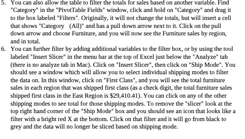
5. You can also allow the table to filter the totals for sales based on another variable. Find "Category" in the "PivotTable Fields" window, click and hold on "Category" and drag it to the box labeled "Filters". Originally, it will not change the totals, but will insert a cell that shows "Category (All)" and has a pull down arrow next to it. Click on the pull down arrow and choose Furniture, and you will now see the Furniture sales by region, and in total. 6. You can further filter by adding additional variables to the filter box, or by using the tool labeled "Insert Slicer" in the menu bar at the top of Excel just below the "Analyze" tab (there is no analyze tab in Mac). Click on "Insert Slicer", then click on "Ship Mode". You should see a window which will allow you to select individual shipping modes to filter the data on. In this window, click on "First Class", and you will see the total furniture sales in each region that was shipped first class (as a check digit, the total furniture sales shipped first class in the East Region is $29,410.41). You can click on any of the other shipping modes to see total for those shipping modes. To remove the "slicer" look at the top right hand corner of the "Ship Mode" box and you should see an icon that looks like a filter with a bright red X at the bottom. Click on that filter and it will go from black to grey and the data will no longer be sliced based on shipping mode