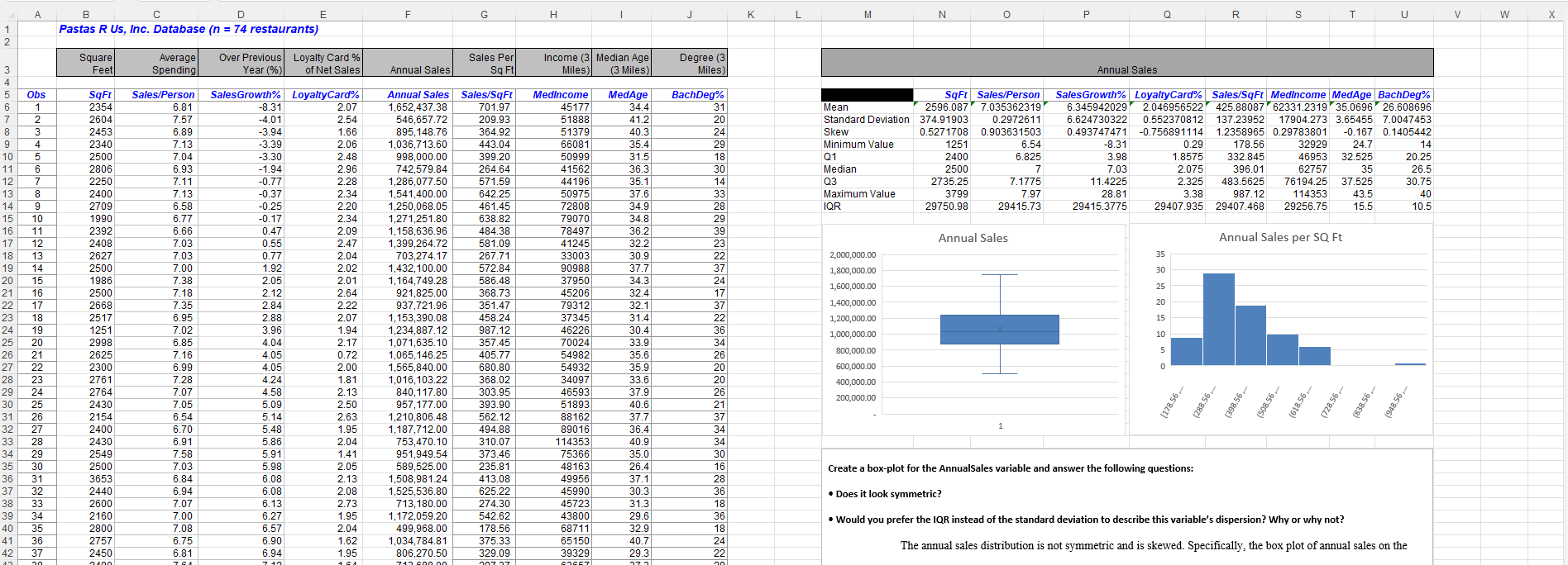
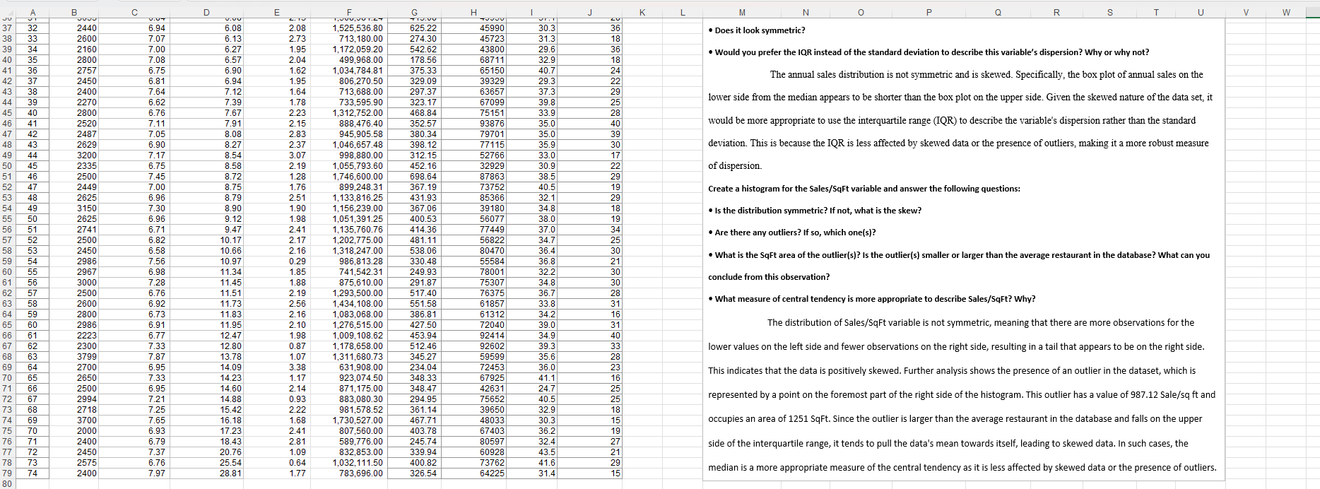
A 1 2 B C D Pastas R Us, Inc. Database (n = 74 restaurants) E F G H J K L M N P R S T U V W X Square 3 Feet Average Spending Over Previous Year (%) Loyalty Card % Sales Per of Net Sales Annual Sales Sq Ft Income (3 Median Age Miles Degree (3 (3 Miles) Miles) Annual Sales 4 5 Obs SqFt Sales/Person SalesGrowth% LoyaltyCard% 6 1 2354 6.81 -8.31 2.07 Annual Sales 1,652,437.38 Sales/SqFt 701.97 Medincome MedAge BachDeg% 45177 34.4 31 Mean SqFt Sales/Person 2596.087 7.035362319 SalesGrowth% Loyalty Card Sales/SqFt Medincome MedAge BachDeg% 6.345942029 2.046956522 425.88087 62331.2319 35.0696 7 2 2604 7.57 -4.01 2.54 546,657.72 209.93 51888 41.2 20 8 3 2453 6.89 -3.94 1.66 895,148.76 364.92 51379 40.3 24 Standard Deviation 374.91903 Skew 9 4 2340 7.13 -3.39 2.06 1,036,713.60 443.04 66081 35.4 29 Minimum Value 0.5271708 1251 0.2972611 0.903631503 6.624730322 0.493747471 0.552370812 137.23952 17904.273 3.65455 -0.756891114 10 5 2500 7.04 -3.30 2.48 998,000.00 399.20 50999 31.5 18 Q1 2400 11 6 2806 6.93 -1.94 2.96 742,579.84 264.64 41562 36.3 30 Median 2500 12 7 2250 7.11 -0.77 2.28 1,286,077.50 571.59 44196 35.1 14 Q3 13 8 2400 7.13 -0.37 2.34 1,541,400.00 642.25 50975 37.6 33 14 9 2709 6.58 -0.25 2.20 1,250,068.05 461.45 72808 34.9 15 10 1990 6.77 -0.17 2.34 1,271,251.80 638.82 79070 34.8 29 16 11 2392 6.66 0.47 2.09 1,158,636.96 484.38 78497 36.2 39 17 12 2408 7.03 0.55 2.47 1,399,264.72 581.09 41245 32.2 18 13 2627 7.03 0.77 2.04 703,274.17 267.71 33003 30.9 19 14 2500 7.00 1.92 2.02 1,432,100.00 572.84 90988 37.7 37 20 15 1986 7.38 2.05 2.01 1,164,749.28 586.48 37950 34.3 24 21 16 2500 7.18 2.12 2.64 921,825.00 368.73 45206 32.4 17 22 17 2668 7.35 2.84 2.22 937,721.96 351.47 79312 32.1 23 18 2517 6.95 2.88 2.07 1,153,390.08 458.24 37345 31.4 24 19 1251 7.02 3.96 1.94 1,234,887.12 987.12 46226 30.4 25 20 2998 6.85 4.04 2.17 1,071,635.10 357.45 70024 33.9 26 21 2625 7.16 4.05 0.72 1,065,146.25 405.77 54982 35.6 27 22 2300 6.99 4.05 2.00 1,565,840.00 680.80 54932 35.9 20 28 23 2761 7.28 4.24 1.81 1,016,103.22 368.02 34097 33.6 29 24 2764 7.07 4.58 2.13 840,117.80 303.95 46593 37.9 322822~2~2832222 Maximum Value IQR 2735.25 3799 29750.98 6.54 6.825 7 7.1775 7.97 29415.73 -8.31 3.98 0.29 1.8575 178.56 332.845 26.608696 7.0047453 1.2358965 0.29783801 -0.167 0.1405442 32929 24.7 46953 32.525 14 20.25 7.03 11.4225 28.81 29415.3775 2.075 2.325 3.38 29407.935 396.01 483.5625 987.12 29407.468 62757 35 26.5 76194.25 114353 29256.75 37.525 30.75 43.5 40 15.5 10.5 Annual Sales Annual Sales per SQ Ft 2,000,000.00 35 30 1,800,000.00 1,600,000.00 25 37 1,400,000.00 20 1,200,000.00 15 36 1,000,000.00 10 34 800,000.00 26 R 1 n 600,000.00 0 20 400,000.00 26 200,000.00 30 25 2430 7.05 5.09 2.50 957,177.00 393.90 51893 40.6 21 31 26 2154 6.54 5.14 2.63 1,210,806.48 562.12 88162 37.7 37 [178.56,... 1 32 27 2400 6.70 5.48 1.95 1,187,712.00 494.88 89016 36.4 34 33 28 2430 6.91 5.86 2.04 753,470.10 310.07 114353 40.9 34 (288.56.... (398.56... (508.56,... (618.56.... (728.56.... (838.56,... (948.56,... 34 29 2549 7.58 5.91 1.41 951,949.54 373.46 75366 35.0 30 35 30 2500 7.03 5.98 2.05 589,525.00 235.81 48163 26.4 16 Create a box-plot for the AnnualSales variable and answer the following questions: 36 31 3653 6.84 6.08 2.13 1,508,981.24 413.08 49956 37.1 28 37 32 2440 6.94 6.08 2.08 1,525,536.80 625.22 45990 30.3 36 Does it look symmetric? 38 33 2600 7.07 6.13 2.73 713,180.00 274.30 45723 31.3 18 39 34 2160 7.00 6.27 1.95 1,172,059.20 542.62 43800 29.6 36 40 35 2800 7.08 6.57 2.04 499,968.00 178.56 68711 32.9 18 41 36 2757 6.75 6.90 1.62 1,034,784.81 375.33 65150 40.7 24 Would you prefer the IQR instead of the standard deviation to describe this variable's dispersion? Why or why not? The annual sales distribution is not symmetric and is skewed. Specifically, the box plot of annual sales on the 42 37 2450 6.81 6.94 1.95 806,270.50 329.09 39329 29.3 22 12 20 0400 764 1.61 710 600.00 007.07 62657 3731 30 A B C D E F G H J K L M N JU 3333 U.UT 0.00 1,000,001.LT +10.00 TOUUD 37 32 2440 6.94 6.08 2.08 1,525,536.80 625.22 45990 30.3 36 Does it look symmetric? 38 33 2600 7.07 6.13 2.73 713,180.00 274.30 45723 31.3 18 39 34 2160 7.00 6.27 1.95 1,172,059.20 542.62 43800 29.6 36 40 35 2800 7.08 6.57 2.04 499,968.00 178.56 68711 32.9 18 41 36 2757 6.75 6.90 1.62 1,034,784.81 375.33 65150 40.7 24 42 37 2450 6.81 6.94 1.95 806,270.50 329.09 39329 29.3 22 43 38 2400 7.64 7.12 1.64 713,688.00 297.37 63657 37.3 29 44 39 2270 6.62 7.39 1.78 733,595.90 323.17 67099 39.8 25 45 40 2800 6.76 7.67 2.23 1,312,752.00 468.84 75151 33.9 28 46 41 2520 7.11 7.91 2.15 888,476.40 352.57 93876 35.0 40 47 42 2487 7.05 8.08 2.83 945,905.58 380.34 79701 35.0 39 48 43 2629 6.90 8.27 2.37 1,046,657.48 398.12 77115 35.9 30 49 44 3200 7.17 8.54 3.07 998,880.00 312.15 52766 33.0 17 50 45 2335 6.75 8.58 2.19 1,055,793.60 452.16 32929 30.9 22 51 46 2500 7.45 8.72 1.28 1,746,600.00 698.64 87863 38.5 29 52 47 2449 7.00 8.75 1.76 899,248.31 367.19 73752 40.5 19 53 48 2625 6.96 8.79 2.51 1,133,816.25 431.93 85366 32.1 29 54 49 3150 7.30 8.90 1.90 1,156,239.00 367.06 39180 34.8 18 55 50 2625 6.96 9.12 1.98 1,051,391.25 400.53 56077 38.0 19 56 51 2741 6.71 9.47 2.41 1,135,760.76 414.36 77449 37.0 34 57 52 2500 6.82 10.17 2.17 1,202,775.00 481.11 56822 34.7 25 58 53 2450 6.58 10.66 2.16 1,318,247.00 538.06 80470 36.4 30 59 54 2986 7.56 10.97 0.29 986,813.28 330.48 55584 36.8 21 60 55 2967 6.98 11.34 1.85 741,542.31 249.93 78001 32.2 30 61 56 3000 7.28 11.45 1.88 875,610.00 291.87 75307 34.8 30 62 57 2500 6.76 11.51 2.19 1,293,500.00 517.40 76375 36.7 28 63 58 2600 6.92 11.73 2.56 1,434,108.00 551.58 61857 33.8 31 64 59 2800 6.73 11.83 2.16 1,083,068.00 386.81 61312 34.2 16 65 60 2986 6.91 11.95 2.10 1,276,515.00 427.50 72040 39.0 31 66 61 2223 6.77 12.47 1.98 1,009,108.62 453.94 92414 34.9 40 67 62 2300 7.33 12.80 0.87 1,178,658.00 512.46 92602 39.3 33 68 63 3799 7.87 13.78 1.07 1,311,680.73 345.27 59599 35.6 28 69 64 2700 6.95 14.09 3.38 631,908.00 234.04 72453 36.0 23 70 65 2650 7.33 14.23 1.17 923,074.50 348.33 67925 41.1 16 71 66 2500 6.95 14.60 2.14 871,175.00 348.47 42631 24.7 25 72 67 2994 7.21 14.88 0.93 883,080.30 294.95 75652 40.5 25 73 68 2718 7.25 15.42 2.22 981,578.52 361.14 39650 32.9 18 74 69 3700 7.65 16.18 1.68 1,730,527.00 467.71 48033 30.3 15 75 70 2000 6.93 17.23 2.41 807,560.00 403.78 67403 36.2 19 76 71 2400 6.79 18.43 2.81 589,776.00 245.74 80597 32.4 27 77 72 2450 7.37 20.76 1.09 832,853.00 339.94 60928 43.5 21 78 73 2575 6.76 25.54 0.64 1,032,111.50 400.82 73762 41.6 29 79 74 2400 7.97 28.81 1.77 783,696.00 326.54 64225 31.4 15 80 P R S T U V W Would you prefer the IQR instead of the standard deviation to describe this variable's dispersion? Why or why not? The annual sales distribution is not symmetric and is skewed. Specifically, the box plot of annual sales on the lower side from the median appears to be shorter than the box plot on the upper side. Given the skewed nature of the data set, it would be more appropriate to use the interquartile range (IQR) to describe the variable's dispersion rather than the standard deviation. This is because the IQR is less affected by skewed data or the presence of outliers, making it a more robust measure of dispersion. Create a histogram for the Sales/SqFt variable and answer the following questions: Is the distribution symmetric? If not, what is the skew? Are there any outliers? If so, which one(s)? What is the SqFt area of the outlier(s)? Is the outlier(s) smaller or larger than the average restaurant in the database? What can you conclude from this observation? What measure of central tendency is more appropriate to describe Sales/SqFt? Why? The distribution of Sales/SqFt variable is not symmetric, meaning that there are more observations for the lower values on the left side and fewer observations on the right side, resulting in a tail that appears to be on the right side. This indicates that the data is positively skewed. Further analysis shows the presence of an outlier in the dataset, which is represented by a point on the foremost part of the right side of the histogram. This outlier has a value of 987.12 Sale/sq ft and occupies an area of 1251 SqFt. Since the outlier is larger than the average restaurant in the database and falls on the upper side of the interquartile range, it tends to pull the data's mean towards itself, leading to skewed data. In such cases, the median is a more appropriate measure of the central tendency as it is less affected by skewed data or the presence of outliers.