Applying Excel $-$ Data Visualization: Excel Worksheet $($Part $1$ of $2)$

Download the Applying Excel form below. Follow the tutorial on the first tab using Excel $\text{'}$s Pivot Table function and Charts.

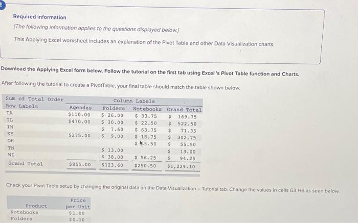
After following the tutorial to create a PivotTable, your final table should match the table shown below.

Sum of Total Order Column Labels

Row Labels Agendas Folders Notebooks Grand Total

IA $ $110\mathrm{.}00$ $ $26\mathrm{.}00$ $ $33\mathrm{.}75$ $ $169\mathrm{.}75$

IL $ $470\mathrm{.}00$ $ $30\mathrm{.}00$ $ $22\mathrm{.}50$ $ $522\mathrm{.}50$

IN $ $7\mathrm{.}60$ $ $63\mathrm{.}75$ $ $71\mathrm{.}35$

KY $ $275\mathrm{.}00$ $ $9\mathrm{.}00$ $ $18\mathrm{.}75$ $ $302\mathrm{.}75$

OH $ $55\mathrm{.}50$ $ $55\mathrm{.}50$

TN $ $13\mathrm{.}00$ $ $13\mathrm{.}00$

WI $ $38\mathrm{.}00$ $ $56\mathrm{.}25$ $ $94\mathrm{.}25$

Grand Total $ $855\mathrm{.}00$ $ $123\mathrm{.}60$ $ $250\mathrm{.}50$ $ $1,229\mathrm{.}10$

Check your Pivot Table setup by changing the original data on the Data Visualization $$ Tutorial tab. Change the values in cells G$3$:H$6$ as seen below.

Product Price

per Unit

Notebooks $ $1\mathrm{.}00$

Folders $ $0\mathrm{.}10$

Agendas $ $4\mathrm{.}50$

After refreshing the Pivot Table data, the total order in KY of folders purchased should be $$4\mathrm{.}50$ and the Grand Total for all states and products should be $$1,165\mathrm{.}30.$

If you did not get these answers, try to refresh the data again for the Pivot Table and follow the tutorial steps again.

Save your completed Applying Excel form to your computer and then upload it here by clicking "Browse". Next click "Save". You will use this worksheet to answer questions in Part $2.$