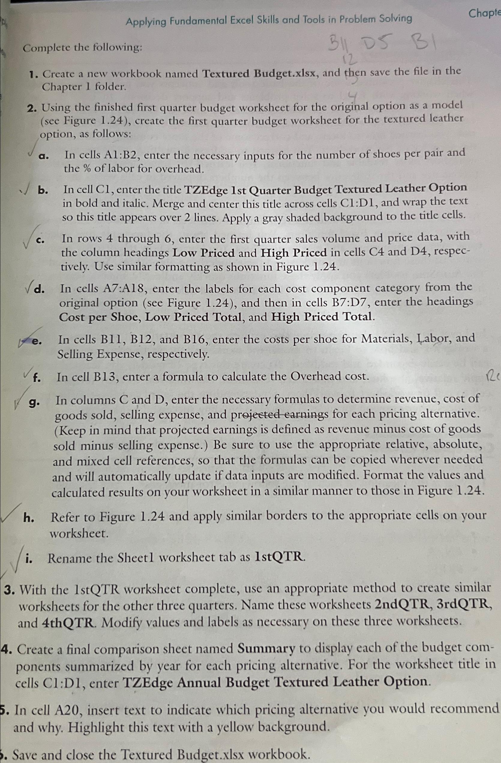
Applying Fundamental Excel Skills and Tools in Problem Solving

Chapte

Complete the following:

$12$

B$)$

Create a new workbook named Textured Budget.xlsx$,$ and then save the file in the Chapter $1$ folder.

Using the finished first quarter budget worksheet for the original option as a model $($see Figure $1\mathrm{.}24),$ create the first quarter budget worksheet for the textured leather option, as follows:

a$.$ In cells $Al$:$B2,$ enter the necessary inputs for the number of shoes per pair and the $\%$ of labor for overhead.

b$.$ In cell Cl$,$ enter the title TZEdge $1$st Quarter Budget Textured Leather Option in bold and italic. Merge and center this title across cells Cl:D$1,$ and wrap the text so this title appears over $2$ lines. Apply a gray shaded background to the title cells.

c$.$ In rows $4$ through $6,$ enter the first quarter sales volume and price data, with the column headings Low Priced and High Priced in cells C$4$ and D$4,$ respectively. Use similar formatting as shown in Figure $1\mathrm{.}24.$

d$.$ In cells A$7$:A$18,$ enter the labels for each cost component category from the original option $($see Figure $1\mathrm{.}24),$ and then in cells B$7$:D$7,$ enter the headings Cost per Shoe, Low Priced Total, and High Priced Total.

e$.$ In cells B$11,$ B$12,$ and B$16,$ enter the costs per shoe for Materials, Labor, and Selling Expense, respectively.

f$.$ In cell B$13,$ enter a formula to calculate the Overhead cost.

g$.$ In columns $C$ and $D,$ enter the necessary formulas to determine revenue, cost of goods sold, selling expense, and prejected earnings for each pricing alternative. $($Keep in mind that projected earnings is defined as revenue minus cost of goods sold minus selling expense.$)$ Be sure to use the appropriate relative, absolute$,$ and mixed cell references, so that the formulas can be copied wherever needed and will automatically update if data inputs are modified. Format the values and calculated results on your worksheet in a similar manner to those in Figure $1\mathrm{.}24.$

h$.$ Refer to Figure $1\mathrm{.}24$ and apply similar borders to the appropriate cells on your worksheet.

i$.$ Rename the Sheetl worksheet tab as IstQTR.

With the $1$stQTR worksheet complete, use an appropriate method to create similar worksheets for the other three quarters. Name these worksheets $2$ndQTR$,3$rdQTR$,$ and $4$thQTR$.$ Modify values and labels as necessary on these three worksheets.

Create a final comparison sheet named Summary to display each of the budget components summarized by year for each pricing alternative. For the worksheet title in cells Cl:D$1,$ enter TZEdge Annual Budget Textured Leather Option.

In cell A$20,$ insert text to indicate which pricing alternative you would recommend and why. Highlight this text with a yellow background.

Save and close the Textured Budget.xlsx workbook.