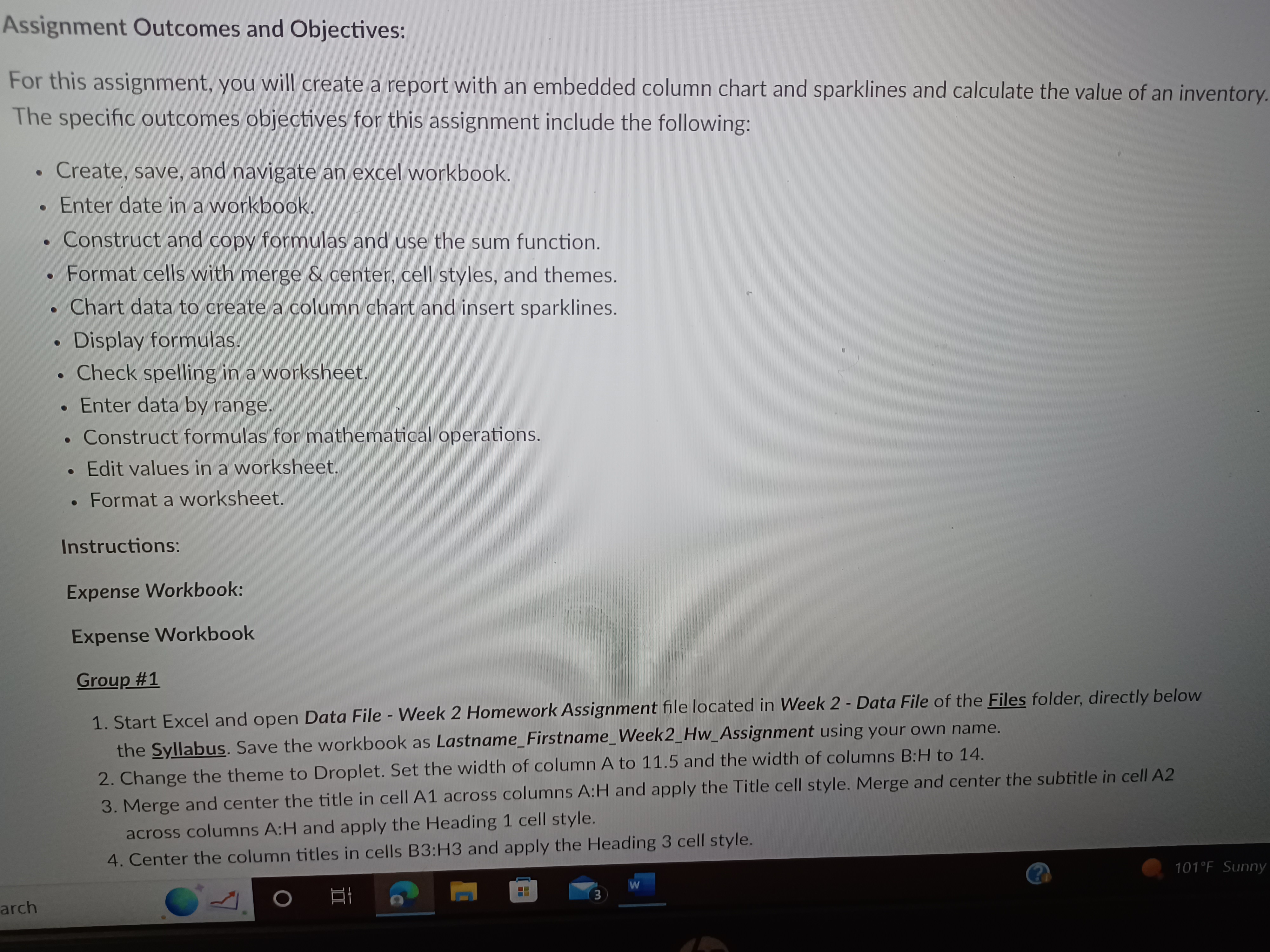
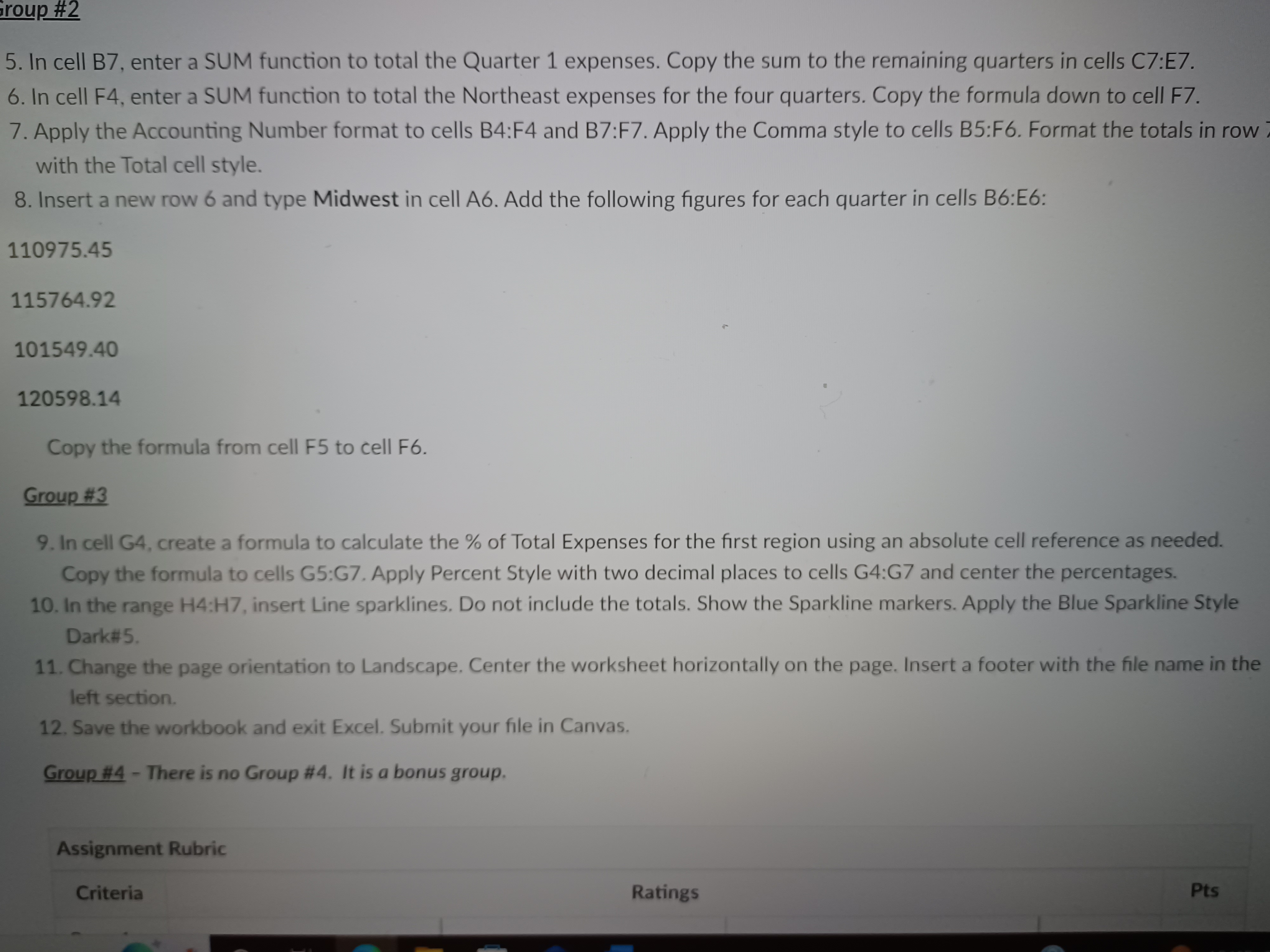
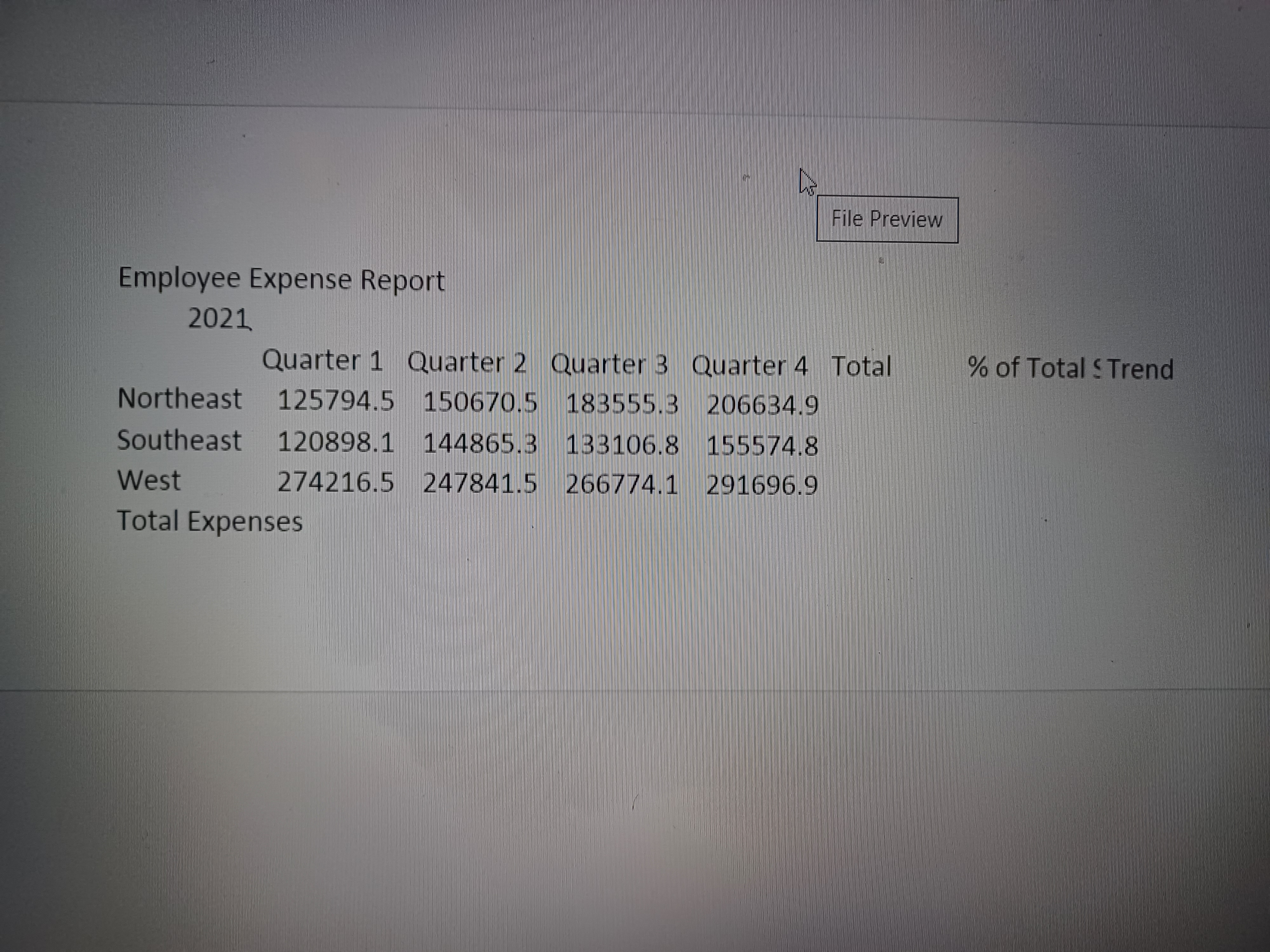
Assignment Outcomes and Objectives: For this assignment, you will create a report with an embedded column chart and sparklines and calculate the value of an inventory. The specific outcomes objectives for this assignment include the following: . Create, save, and navigate an excel workbook. . Enter date in a workbook. . Construct and copy formulas and use the sum function. . Format cells with merge & center, cell styles, and themes. . Chart data to create a column chart and insert sparklines. . Display formulas. . Check spelling in a worksheet. . Enter data by range. . Construct formulas for mathematical operations. . Edit values in a worksheet. . Format a worksheet. Instructions: Expense Workbook: Expense Workbook Group #1 1. Start Excel and open Data File - Week 2 Homework Assignment file located in Week 2 - Data File of the Files folder, directly below the Syllabus. Save the workbook as Lastname_Firstname_Week2_Hw_Assignment using your own name. 2. Change the theme to Droplet. Set the width of column A to 11.5 and the width of columns B:H to 14. 3. Merge and center the title in cell A1 across columns A:H and apply the Title cell style. Merge and center the subtitle in cell A2 across columns A:H and apply the Heading 1 cell style. 4. Center the column titles in cells B3:H3 and apply the Heading 3 cell style. 101 F Sunny arch Oroup #2 5. In cell B7, enter a SUM function to total the Quarter 1 expenses. Copy the sum to the remaining quarters in cells C7:E7. 6. In cell F4, enter a SUM function to total the Northeast expenses for the four quarters. Copy the formula down to cell F7. 7. Apply the Accounting Number format to cells B4:F4 and B7:F7. Apply the Comma style to cells B5:F6. Format the totals in row with the Total cell style. 8. Insert a new row 6 and type Midwest in cell A6. Add the following figures for each quarter in cells B6:E6: 110975.45 115764.92 101549.40 120598.14 Copy the formula from cell F5 to cell F6. Group #3 9. In cell G4, create a formula to calculate the % of Total Expenses for the first region using an absolute cell reference as needed. Copy the formula to cells G5:G7. Apply Percent Style with two decimal places to cells G4:G7 and center the percentages. 10. In the range H4:H7, insert Line sparklines. Do not include the totals. Show the Sparkline markers. Apply the Blue Sparkline Style Dark#5. 11. Change the page orientation to Landscape. Center the worksheet horizontally on the page. Insert a footer with the file name in the left section. 12. Save the workbook and exit Excel. Submit your file in Canvas. Group #4 - There is no Group #4. It is a bonus group. Assignment Rubric Criteria Ratings PtsFile Preview Employee Expense Report 2021 Quarter 1 Quarter 2 Quarter 3 Quarter 4 Total % of Total S Trend Northeast 125794.5 150670.5 183555.3 206634.9 Southeast 120898.1 144865.3 133106.8 155574.8 West 274216.5 247841.5 266774.1 291696.9 Total Expenses