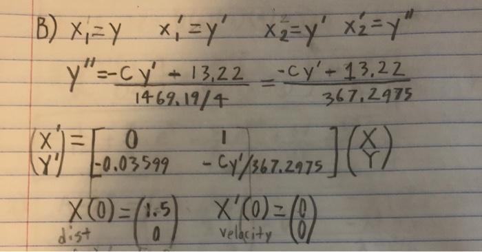
nd C) Use the IVP Solver script in MATLAB to plot solutions to your system with small, varying choices of the damping coefficient c. Use the hold on command to plot many different solution curves on the same set of axes. Provide your plot and code in your final submission. Leave comments noting what values of c were used in the script. Now, select an appropriate choice for c, based on your results above, that causes no more than two oscillations of the vehicle. This will be your damping coefficient for the remainder of the project. D) Create a phase portrait of your first order system using the Phase Portrait script in MATLAB. Provide your plot and code in your final submission. Classify the type and stability of the critical point at the origin, then describe why your phase portrait matches your solution determined using the IVP Solver. B) x = Y x = y X =Y X =Y" y"=-cy' 13,22 1469.19/4 -Cy'-13.22 367,2975 I -0.03599 - Cy/367.2975 - CY/367.2975 ] (X) X(0) = (8) velocity x = 0 Y X (0)= (1.5) dist