Can you help me understand this Satistic problem? Last week's discussion involved development of a multiple regression model that used miles per gallon as a response variable. Weight and horsepower were predictor variables. You performed an overall F-test to evaluate the significance of your model. This week, you will evaluate the significance of individual predictors. Is at least one of the two variables (weight and horsepower) significant in the model? Run the overall F-test and provide your interpretation at 5% level of significance.

1. Define the null and alternative hypothesis in mathematical terms and in words.
2. What is the slope coefficient for the weight variable? Is this coefficient significant at 5% level of significance (alpha=0.05)? (Hint: Check the P-value,p>|t|, for weight in Python output. Recall that this is the individual t-test for the beta parameter.)
3. What is the slope coefficient for the horsepower variable? Is this coefficient significant at 5% level of significance (alpha=0.05)? (Hint: Check the P-value,p>|t|, for horsepower in Python output. Recall that this is the individual t-test for the beta parameter.

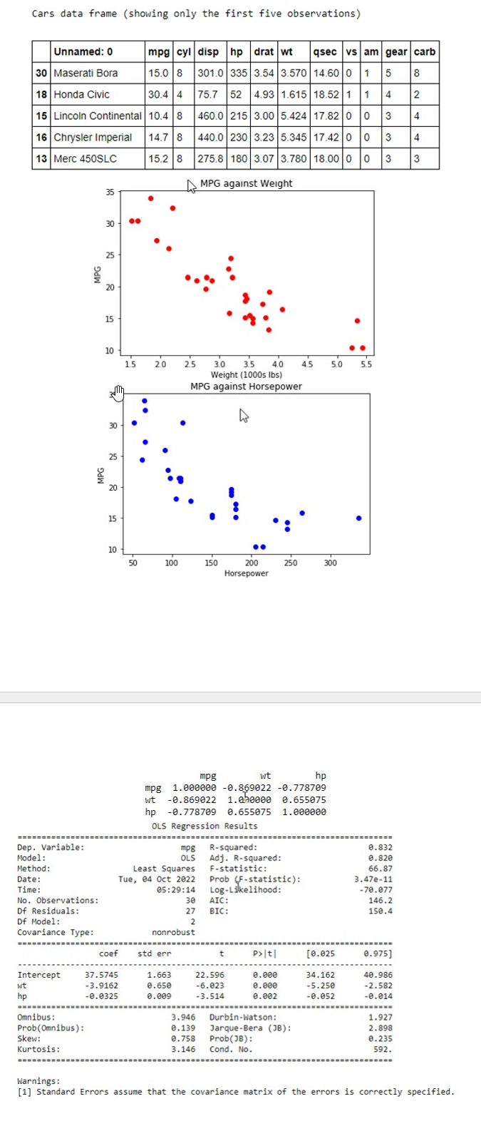
Cars data frame (showing only the first five observations) Unnamed: 0 mpg cyl disp hp drat wt qsec am gear carb 30 Maserati Bora 15.0 8 301.0 335 3.54 3.570 14.60 0 1 8 Honda Civic 30.4 14 75,7 52 1.93 1.615 18.52 15 Lincoln Continental 10.4 460.0 215 3.00 5.424 17.82 10 0 3 16 Chrysler Imperial 14.7 8 440.0 230 3.23 5.345 17.42 0 0 3 4 13 Merc 450SLC 15.2 8 275.8 180 3.07 3.780 18.00 0 10 3 MPG against Weight 35 30 MPG 20 15 . . 10 15 20 25 3.0 35 40 4.5 5.0 5.5 Weight (1000s lbs) MPG against Horsepower . . 30 MPG 20 . .. 15 . 10 .. 50 100 150 200 250 300 Horsepower mpg wt hp mpg 1.000000 -0.869022 -0.778709 wit SLoss9 0 0oo060.T 270698 0- hp -0.778709 0.655075 1.000000 OLS Regression Results Dep. Variable: mpg R-squared: 0.832 Model : OLS Adj. R-squared: 0. 820 Method : Least Squares F-statistic: 66.87 Date: Tue, 04 Oct 2022 Prob (F-statistic) : 3.47e-11 Time : 05:29:14 Log-Likelihood: -70.077 No. Observations: 30 AIC 146.2 Of Residuals: 27 BIC: 150.4 Of Model: Covariance Type: nonrobust coef std err P>t [0.025 0.975] Intercept 37.5745 1.663 22.596 0.0ee 34.162 40.986 wt -3.9162 0.650 -6.023 0.0ee -5.250 -2.582 hp -0.0325 0.009 -3.514 0. 002 -0.052 -0.014 Omnibus 3.946 Durbin-Watson: 1.927 Prob(Omnibus) : 3.139 Jarque-Bera (JB) : 2.898 Skew: 0.758 Prob(JB) : 0.235 Kurtosis : 3.146 Cond. No. 592. Warnings: [1] Standard Errors assume that the covariance matrix of the errors is correctly specified