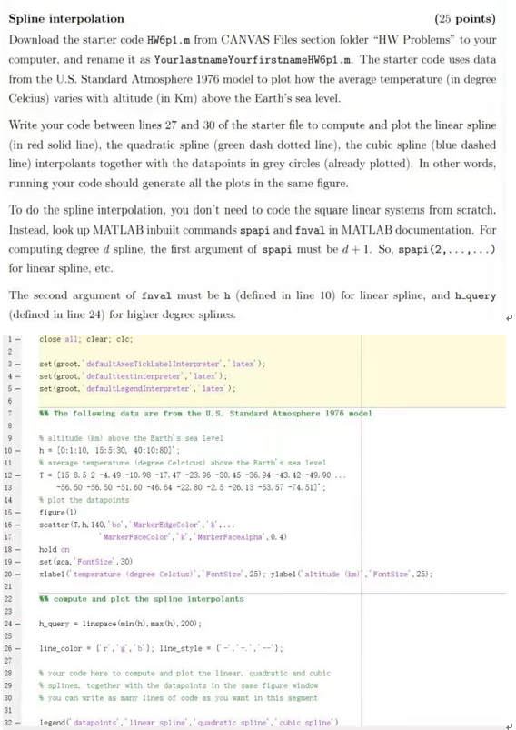
close all; clear; clc;

set(groot,'defaultAxesTickLabelInterpreter','latex'); set(groot,'defaulttextinterpreter','latex'); set(groot,'defaultLegendInterpreter','latex');

%% The following data are from the U.S. Standard Atmosphere 1976 model

% altitude (km) above the Earth's sea level h = [0:1:10, 15:5:30, 40:10:80]'; % average temperature (degree Celcicus) above the Earth's sea level T = [15 8.5 2 -4.49 -10.98 -17.47 -23.96 -30.45 -36.94 -43.42 -49.90 ... -56.50 -56.50 -51.60 -46.64 -22.80 -2.5 -26.13 -53.57 -74.51]'; % plot the datapoints figure(1) scatter(T,h,140,'bo','MarkerEdgeColor','k',... 'MarkerFaceColor','k','MarkerFaceAlpha',0.4) hold on set(gca,'FontSize',30) xlabel('temperature (degree Celcius)','FontSize',25); ylabel('altitude (km)','FontSize',25);

%% compute and plot the spline interpolants

h_query = linspace(min(h),max(h),200);

line_color = {'r','g','b'}; line_style = {'-','-.','--'};

% your code here to compute and plot the linear, quadratic and cubic % splines, together with the datapoints in the same figure window % you can write as many lines of code as you want in this segment

legend('datapoints','linear spline','quadratic spline','cubic spline')