code

# -*- coding: utf-8 -*- """ Spyder Editor

This is a temporary script file. """ from mpl_toolkits.basemap import Basemap from netCDF4 import Dataset

import matplotlib.pyplot as plt import numpy as np

fIn = '/Users/Ajda/Documents/UW/TA-ATMS301/Labs/Lab_06_imgs/ERA5_20180104.nc'

# # # read in data data = Dataset(fIn, 'r') longitude = np.array(data['longitude']) latitude = np.flip(np.array(data['latitude']), 0) pressure = np.array(data['level']) geopotential = np.flip(np.array(data['z']), 2) cloud_cov = np.flip(np.array(data['cc']), 2) t = np.flip(np.array(data['t']), 2) data.close()

# # # create a grid with latitude and longitude coordinates lonGrid, latGrid = np.meshgrid(longitude, latitude) # # # let's see what the area of data we have is bounded by print('Minimum longitude: ', longitude.min()) print('Maximum longitude: ', longitude.max()) print('Minimum latitude: ', latitude.min()) print('Maximum latitude: ', latitude.max())

# # # Some useful calculations z = geopotential / 9.81 print('Dimensions of z:', z.shape) # dimensions of height array # # # (4, 37, 181, 381) - (time, level, latitude, longitude) # # # calculate the Coriolis force parameter f = 2 * (7.292 * 10**(-5)) * np.sin(np.deg2rad(latGrid)) print('Dimensions of f:', f.shape) # dimensions of height array

# # # space for some data manipulation here # EXAMPLE 1: Averaging along a dimension

# EXAMPLE 2: Averaging neighboring elements

# EXAMPLE 3: Calculating gradients

# # # Calculate geostrophic winds

# # # define a map m = Basemap(width=7100000, height=5000000, rsphere=(6378137.00,6356752.3142), \ resolution='l', area_thressh=1000., projection='lcc', lat_1=30., \ lat_2=55, lat_0=40, lon_0=-85.) # # # transform the lat-lon coordinates to the right projection (Lambert Conformal) lonG, latG = m(lonGrid, latGrid)

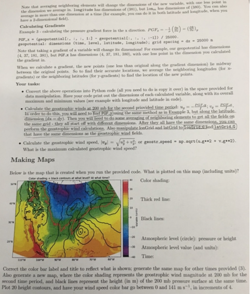
# # # plot figure fig = plt.figure(figsize = (10, 6)) # # # create axes ax = fig.add_subplot(111) # # # draw the map in the background m.drawcoastlines(ax=ax, linewidth=.5) m.drawcountries(ax=ax, linewidth=.2) m.drawstates(ax=ax, linewidth=.2) m.drawmeridians(np.arange(-150, 20, 10), linewidth=.3, labels=[0, 0, 0, 1]) m.drawmeridians(np.arange(-155, 20, 10), linewidth=.3) m.drawparallels(np.arange(10, 90, 10), linewidth=.3, labels=[1, 0, 0, 0]) m.drawparallels(np.arange(15, 90, 10), linewidth=.3) # # # plot some data f1 = m.contourf(lonG, latG, t[0][-1]-273.15, np.arange(-40, 40.1, 2), cmap='nipy_spectral') m.contour(lonG, latG, t[0][-1]-273.15, levels=[0], colors='r', linewidths=3) m.contour(lonG, latG, geopotential[0][-1]/9.81, levels=np.arange(-100, 300, 50), colors='k', linewidths=2, linestyles='solid') m.colorbar(f1, label='Variable (units)') ax.set_title('Color shading + black contours at what level? At what time?') plt.savefig('/Users/Ajda/Documents/UW/TA-ATMS301/Labs/Lab_06_imgs/Img01.png', dpi=200, bbox_inches='tight') plt.close()

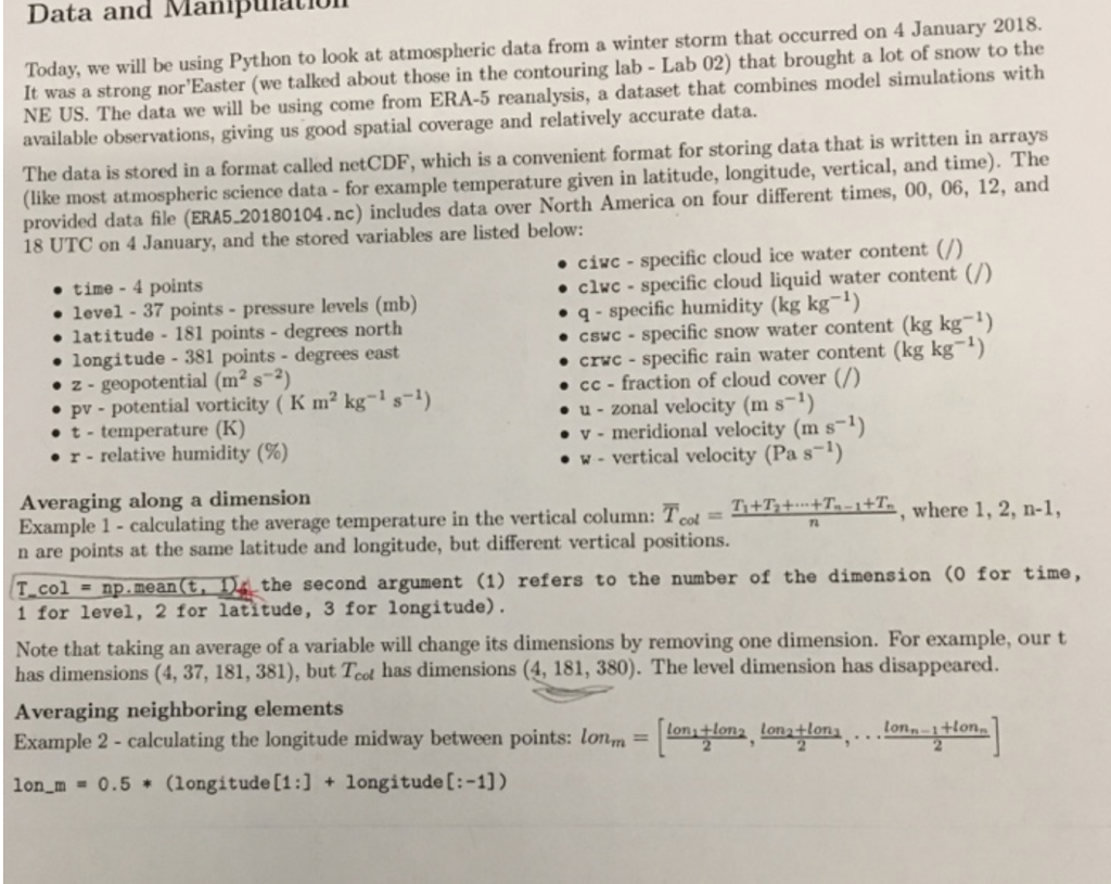
Data and ManlpuiatioI Today, we will be using Python to look at atmospheric data from a winter storm that occurred on 4 January 2018. It was a strong nor Easter (we talked about those in the contouring lab - Lab 02) that brought a lot of snow to the NE US. The data we will be using come from ERA-5 reanalysis, a dataset that combines model simulations with available observations, giving us good spatial coverage and relatively accurate data. The data is stored in a format called netCDF, which is a convenient format for storing data that is written in arrays (like most atmospheric science data-for example temperature given in latitude, longitude, vertical, and time). The provided data file (ERA5.20180104.nc) includes data over North America on four different times, 00, 06, 12, and 18 UTC on 4 January, and the stored variables are listed below: time-4 points level-37 points- pressure levels (mb) latitude-181 points - degrees north longitude-381 points - degrees east ciuc-specific cloud ice water content (/) cluc-specific cloud liquid water content (/) q-specific humidity (kg kg-) cswc-specific snow water content ( kg-1) cruc-specific rain water content (kg kg-1) . z-geopotential (m2 s2) cc-fraction of cloud cover (/) pv - potential vorticity (K m2 kg-s-1) t-temperature (K) u- zonal velocity (m s-1) v-meridional velocity (m s-1) w-vertical velocity (Pa s-) r-relative humidity (%) A veraging along a dimension Example 1 - calculating the average temperature in the vertical column: T n are points at the same latitude and longitude, but different vertical positions. TT, where 1, 2, n-1, T.col-np.mean 1 for level, 2 for latitude, 3 for longitude) the second argument (1) reters to the number of the dimension (o for time, Note that taking an average of a variable will change its dimensions by removing one dimension. For example, our t has dimensions (4, 37, 181, 381), but Teot has dimensions (4, 181, 380). The level dimension has disappeared. Averaging neighboring elements Example 2 - calculating the longitude midway between points: lonmlomtlon, mlon Ion-m= 0.5 * (longitude [1:] + longitude [:-1]) ona ton Data and ManlpuiatioI Today, we will be using Python to look at atmospheric data from a winter storm that occurred on 4 January 2018. It was a strong nor Easter (we talked about those in the contouring lab - Lab 02) that brought a lot of snow to the NE US. The data we will be using come from ERA-5 reanalysis, a dataset that combines model simulations with available observations, giving us good spatial coverage and relatively accurate data. The data is stored in a format called netCDF, which is a convenient format for storing data that is written in arrays (like most atmospheric science data-for example temperature given in latitude, longitude, vertical, and time). The provided data file (ERA5.20180104.nc) includes data over North America on four different times, 00, 06, 12, and 18 UTC on 4 January, and the stored variables are listed below: time-4 points level-37 points- pressure levels (mb) latitude-181 points - degrees north longitude-381 points - degrees east ciuc-specific cloud ice water content (/) cluc-specific cloud liquid water content (/) q-specific humidity (kg kg-) cswc-specific snow water content ( kg-1) cruc-specific rain water content (kg kg-1) . z-geopotential (m2 s2) cc-fraction of cloud cover (/) pv - potential vorticity (K m2 kg-s-1) t-temperature (K) u- zonal velocity (m s-1) v-meridional velocity (m s-1) w-vertical velocity (Pa s-) r-relative humidity (%) A veraging along a dimension Example 1 - calculating the average temperature in the vertical column: T n are points at the same latitude and longitude, but different vertical positions. TT, where 1, 2, n-1, T.col-np.mean 1 for level, 2 for latitude, 3 for longitude) the second argument (1) reters to the number of the dimension (o for time, Note that taking an average of a variable will change its dimensions by removing one dimension. For example, our t has dimensions (4, 37, 181, 381), but Teot has dimensions (4, 181, 380). The level dimension has disappeared. Averaging neighboring elements Example 2 - calculating the longitude midway between points: lonmlomtlon, mlon Ion-m= 0.5 * (longitude [1:] + longitude [:-1]) ona ton