Consider the system shown in Figure $3.$ The system is at

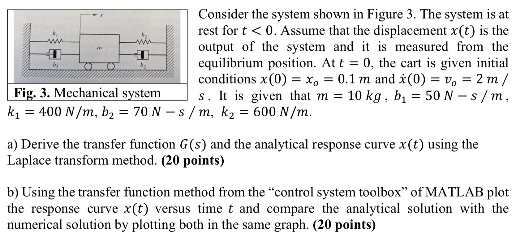
rest for Assume that the displacement $x(t)$ is the

output of the system and it is measured from the

equilibrium position. At $t=0,$ the cart is given initial

conditions $x(0)=x_o=0\mathrm{.}1m$ and $x^{}(0)=v_o=2\frac{m}{?}$

$s.$ It is given that $m=10kg,b_1=50N-\frac{s}{m},$

$k_1=400\frac{N}{m},b_2=70N-\frac{s}{m},k_2=600\frac{N}{m}.$

a$)$ Derive the transfer function $G(s)$ and the analytical response curve $x(t)$ using the

Laplace transform method. $(20$ points$)$

b$)$ Using the transfer function method from the "control system toolbox" of MATLAB plot

the response curve $x(t)$ versus time $t$ and compare the analytical solution with the

numerical solution by plotting both in the same graph. $(20$ points$)$