Constructing the Non-Linear Model You must call the function nonlinear.m in order to produce a non-linear estimate of the variables h, , u and at time-level m + 1,

how do you set up the call tree for it?How do you create this while loop ?

the nonlinear function:

[u1,h1,eta1] = gravity(u1,h1,eta1,N,dx,dt,g,H);

 % cell-center values from cell-edge values % flow and surface uc1 = (u1(1:N)+u1(2:N+1))/2; hc1 = (h1(1:N)+h1(2:N+1))/2; % mass flux U1 = u1.*h1; Uc1 = (U1(1:N)+U1(2:N+1))/2; % tracer phic1 = (phi1(1:N)+phi1(2:N+1))/2; % % % advect mass, mass flux and tracer [hc2] = FCT(hc1,uc1,dx,N,dt); [Uc2] = FCT(Uc1,uc1,dx,N,dt); [phic2] = FCT(phic1,uc1,dx,N,dt); uc2 = Uc2./hc2; % % % % edge-values from cell-centered values % surface h2(2:N) = (hc2(1:N-1)+hc2(2:N))/2; % BCs h2(1) = h2(2); h2(N+1) = h2(N); % momentum u2(2:N) = (uc2(1:N-1)+uc2(2:N))/2; % BCs u2(1) = 0; u2(N+1) = 0; % tracer phi2(2:N) = (phic2(1:N-1)+phic2(2:N))/2; % BCs phi2(1) = phi2(2); phi2(N+1) = phi2(N); eta2 = h2-H; end function [q2]=FCT(q1,u,dx,N,dt); % 1-D advection of tracer following % the flux conservation law dq/dt + d(uq)/dx = 0 % by flux corrected transport/flux limiter method % with superbee limiter, no-flux boundary conditions % % q1: initial distribution of q (cell-centered) % q2: distribution after dt seconds (cell-centered) % u: advecting flow speed (cell-centered) % dt: time step % dx: cell width % N: length of arrays % N cells, N+1 edges/fluxes % umh = flow speed at cell edge n-1/2 % f(1) = 0; for n=2:N if n==N ii = [N-2 N-1 N N]; umh = (u(N-1)+u(N))/2; elseif n==2 ii = [1 1 2 3]; umh = (u(1)+u(2))/2; else ii = [n-2 n-1 n n+1]; umh = (u(n-1)+u(n))/2; end [f(n)] = flux(umh,q1(ii),dx,dt); end f(N+1) = 0; q2 = q1 - (dt/dx).*(f(2:N+1)'-f(1:N)'); end function [f] = flux(u,q,dx,dt); % USAGE: [f] = flux(u,q,dx,dt) % u = left-cell-edge flow u_{n-1/2} % q = flux-conserved quantity (4-point stencil, cell centered) % dx, dt = cell width, time interval % superbee flux limiter if u>=0 r = (q(2)-q(1))/(q(3)-q(2)); else r = (q(4)-q(3))/(q(3)-q(2)); end phi = max([0 min(1,2*r) min(2,r)]); f = ( ... 0.5*( (1+sign(u))*q(2)*u ... +(1-sign(u))*q(3)*u ) ... + 0.5*abs(u)*(1-abs(u*dt/dx))*phi*(q(3)-q(2)) ... ); end

Gravity function :

% Inputs: % u1 - flow speed at nodes, time level 1 (N+1) X 1 % eta1 - surface elevation at nodes, time level 1 (N+1) X 1 % h1 - surface elevation at nodes, time level 1 (N+1) X 1 % N,dx,dt,g,H - array size, grid size, time step, gravity, % mean depth 1 X 1 % % Outputs: % u2 - flow speed at nodes, time level 2 after dt (N+1) X 1 % eta2 - surface elevation at nodes, time level 2 after dt (N+1) X 1 % h2 - surface elevation at nodes, time level 2 after dt (N+1) X 1 % % check sizes of input arguments, return error if sum([size(dx)~=[1 1] size(N)~=[1 1] size(dt)~=[1 1] size(g)~=[1 1] size(H)~=[1 1]]) error('ERROR: one or more of dx, N, dt, g, H is not scalar'); elseif sum([size(u1)~=[N+1 1] size(eta1)~=[N+1 1] size(h1)~=[N+1 1]]) error('One or more vector input arguments are wrong size'); else end % construct A,b A = zeros(2*(N+1)); b = zeros(2*(N+1),1); % u on boundaries b(1) = 0; A(1,1) = 1; b(N+1) = 0; A(N+1,N+1) = 1; % eta on boundaries b((N+1)+1) = 0; A((N+1)+1,(N+1)+1) = 1; A((N+1)+1,(N+1)+2) = -1; b(2*(N+1)) = 0; A(2*(N+1),2*(N+1)) = 1; A(2*(N+1),2*(N+1)-1) = -1; for n=2:N % u interior b(n) = u1(n); A(n,n) = 1; A(n,(N+1)+(n-1)) = -g*dt/(2*dx); A(n,(N+1)+(n+1)) = g*dt/(2*dx); % eta interior b((N+1)+n) = eta1(n); A((N+1)+n,(N+1)+n) = 1; A((N+1)+n,n-1) = -H*dt/(2*dx); A((N+1)+n,n+1) = H*dt/(2*dx); end % solve Ax=b x = A; % decompose u, eta u2 = x(1:N+1); eta2 = x(N+2:2*(N+1)); h2 = eta2+H; end

Transport function

ttf = [ -1 1 0 0 0; 0 1/8 1/16 0 0 ; 0 -1/8 1 1/8 0 ; 0 0 -1/16 7/8 1/8 ; 0 0 0 -1 1 ]

w = [ 0 1/2 1 1/2 0]'

ttf * w = b

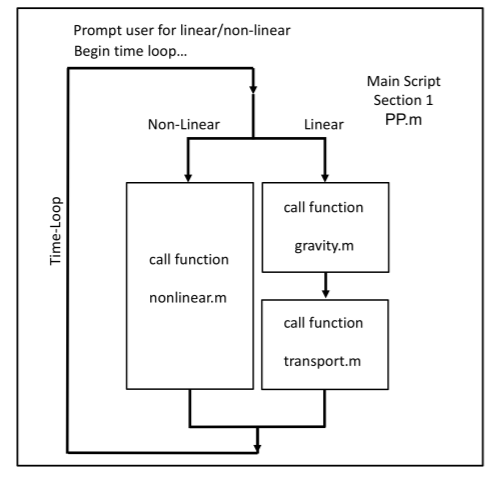
Prompt user for linearon-linear Begin time loop... Main Script Section 1 PP.m Non-Linear Linear call function gravity.nm call function nonlinear.m call function transport.m Prompt user for linearon-linear Begin time loop... Main Script Section 1 PP.m Non-Linear Linear call function gravity.nm call function nonlinear.m call function transport.m