

Question: Course: QUAL8115 - Advanced design of Experiments Assignment 4 - RSM & Optimization In this assignment you are provided information on an experiment and you
Course: QUAL8115 - Advanced design of Experiments
Assignment 4 - RSM & Optimization
In this assignment you are provided information on an experiment and you are required to investigate and interpret the output which is provided below.
Problem:Consider the three?variable central composite design shown in the table.
| RunOrder | PtType | Blocks | Temperature | Time | Catalyst | Conversion (%) y1 | Viscosity y2 |
| 1 | 1 | 1 | -1 | -1 | -1 | 74 | 53.2 |
| 2 | 1 | 1 | 1 | -1 | -1 | 51 | 62.9 |
| 3 | 1 | 1 | -1 | 1 | -1 | 88 | 53.4 |
| 4 | 1 | 1 | 1 | 1 | -1 | 70 | 62.6 |
| 5 | 1 | 1 | -1 | -1 | 1 | 71 | 57.3 |
| 6 | 1 | 1 | 1 | -1 | 1 | 90 | 67.9 |
| 7 | 1 | 1 | -1 | 1 | 1 | 66 | 59.8 |
| 8 | 1 | 1 | 1 | 1 | 1 | 97 | 67.8 |
| 9 | -1 | 1 | -1.68179 | 0 | 0 | 76 | 59.1 |
| 10 | -1 | 1 | 1.681793 | 0 | 0 | 79 | 65.9 |
| 11 | -1 | 1 | 0 | -1.68179 | 0 | 85 | 60 |
| 12 | -1 | 1 | 0 | 1.681793 | 0 | 97 | 60.7 |
| 13 | -1 | 1 | 0 | 0 | -1.68179 | 55 | 57.4 |
| 14 | -1 | 1 | 0 | 0 | 1.681793 | 81 | 63.2 |
| 15 | 0 | 1 | 0 | 0 | 0 | 81 | 59.2 |
| 16 | 0 | 1 | 0 | 0 | 0 | 75 | 60.4 |
| 17 | 0 | 1 | 0 | 0 | 0 | 76 | 59.1 |
| 18 | 0 | 1 | 0 | 0 | 0 | 83 | 60.6 |
| 19 | 0 | 1 | 0 | 0 | 0 | 80 | 60.8 |
| 20 | 0 | 1 | 0 | 0 | 0 | 91 | 58.9 |
Modified fromDesign and Analysis of Experiments (9th Edition) [Texidium version]. (2017). Retrieved fromhttp://texidium.com
Part 1- Conversion percent
A partial Minitab output for the full model is shown below.
Model Summary
| S | R-sq | R-sq(adj) | R-sq(pred) |
| 4.71669 | 91.99% | 84.79% | 75.66% |
Fits and Diagnostics for Unusual Observations
| Obs | Conversion % (y1) | Fit | Resid | Std Resid | |
| 20 | 91.00 | 81.09 | 9.91 | 2.30 | R |
R Large residual
Analysis of Variance
| Source | DF | Adj SS | Adj MS | F-Value | P-Value |
| Model | 9 | 2555.73 | 283.97 | 12.76 | 0.000 |
| Linear | 3 | 763.05 | 254.35 | 11.43 | 0.001 |
| Temperature | 1 | 14.44 | 14.44 | 0.65 | 0.439 |
| Time | 1 | 222.96 | 222.96 | 10.02 | 0.010 |
| Catalyst | 1 | 525.64 | 525.64 | 23.63 | 0.001 |
| Square | 3 | 601.30 | 200.43 | 9.01 | 0.003 |
| Temperature*Temperature | 1 | 48.47 | 48.47 | 2.18 | 0.171 |
| Time*Time | 1 | 124.48 | 124.48 | 5.60 | 0.040 |
| Catalyst*Catalyst | 1 | 388.59 | 388.59 | 17.47 | 0.002 |
| 2-Way Interaction | 3 | 1191.37 | 397.12 | 17.85 | 0.000 |
| Temperature*Time | 1 | 36.12 | 36.12 | 1.62 | 0.231 |
| Temperature*Catalyst | 1 | 1035.12 | 1035.12 | 46.53 | 0.000 |
| Time*Catalyst | 1 | 120.13 | 120.13 | 5.40 | 0.043 |
| Error | 10 | 222.47 | 22.25 | ||
| Lack-of-Fit | 5 | 56.47 | 11.29 | 0.34 | 0.869 |
| Pure Error | 5 | 166.00 | 33.20 | ||
| Total | 19 | 2778.20 |
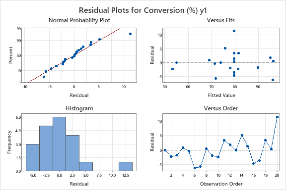
Interpret the above output. As well as discussing factor significance you are expected to discuss the unusual residual and how it may (or may not) affect the overall analysis. Is there a specific recommendation that you would make?
The partial output for the reduced model is provided.
Model Summary
| S | R-sq | R-sq(adj) | R-sq(pred) |
| 5.05856 | 88.95% | 82.50% | 69.18% |
Coded Coefficients
| Term | Coef | SE Coef | T-Value | P-Value | VIF |
| Constant | 79.59 | 1.75 | 45.45 | 0.000 | |
| Temperature | 1.03 | 1.37 | 0.75 | 0.467 | 1.00 |
| Time | 4.04 | 1.37 | 2.95 | 0.012 | 1.00 |
| Catalyst | 6.20 | 1.37 | 4.53 | 0.001 | 1.00 |
| Time*Time | 3.12 | 1.33 | 2.35 | 0.036 | 1.01 |
| Catalyst*Catalyst | -5.01 | 1.33 | -3.78 | 0.003 | 1.01 |
| Temperature*Catalyst | 11.37 | 1.79 | 6.36 | 0.000 | 1.00 |
| Time*Catalyst | -3.88 | 1.79 | -2.17 | 0.051 | 1.00 |
Analysis of Variance
| Source | DF | Adj SS | Adj MS | F-Value | P-Value |
| Model | 7 | 2471.13 | 353.02 | 13.80 | 0.000 |
| Linear | 3 | 763.05 | 254.35 | 9.94 | 0.001 |
| Temperature | 1 | 14.44 | 14.44 | 0.56 | 0.467 |
| Time | 1 | 222.96 | 222.96 | 8.71 | 0.012 |
| Catalyst | 1 | 525.64 | 525.64 | 20.54 | 0.001 |
| Square | 2 | 552.83 | 276.42 | 10.80 | 0.002 |
| Time*Time | 1 | 141.78 | 141.78 | 5.54 | 0.036 |
| Catalyst*Catalyst | 1 | 365.42 | 365.42 | 14.28 | 0.003 |
| 2-Way Interaction | 2 | 1155.25 | 577.62 | 22.57 | 0.000 |
| Temperature*Catalyst | 1 | 1035.12 | 1035.12 | 40.45 | 0.000 |
| Time*Catalyst | 1 | 120.13 | 120.13 | 4.69 | 0.051 |
| Error | 12 | 307.07 | 25.59 | ||
| Lack-of-Fit | 7 | 141.07 | 20.15 | 0.61 | 0.736 |
| Pure Error | 5 | 166.00 | 33.20 | ||
| Total | 19 | 2778.20 |
![and Analysis of Experiments (9th Edition) [Texidium version]. (2017). Retrieved fromhttp://texidium.comPart 1-](https://s3.amazonaws.com/si.experts.images/answers/2024/06/667e83ef47fd5_343667e83ef21cc3.jpg)
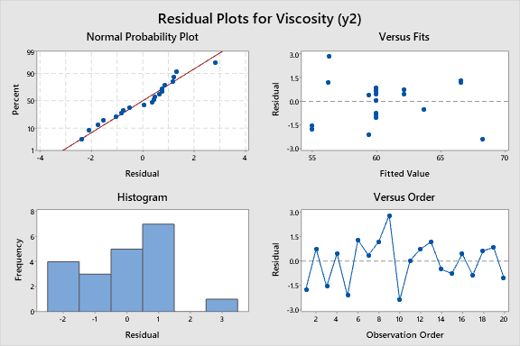
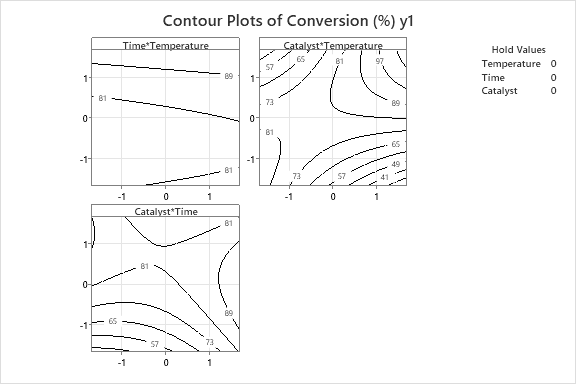
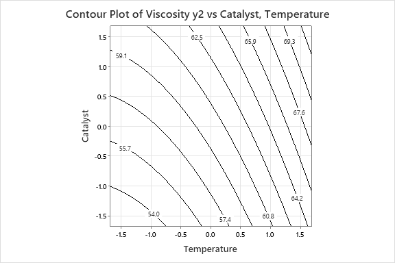
Residual Plots for Conversion (%) y1 Normal Probability Plot Versus Fits 10 90 Percent 50 Residual 10 10 50 70 90 Residual Fitted Value Histogram Versus Order 10 4.5 Frequency 3.0 Residual 1.5 -S -5.0 -2.5 0.0 2.5 5.0 7.5 10.0 12.5 2 4 6 10 12 14 16 18 20 Residual Observation OrderResidual Plots for Viscosity (y2) Normal Probability Plot Versus Fits 3.0 1.5 Percent 50 Residual 10 -1.5 -3.0 4 SE 70 Residual Fitted Value Histogram Versus Order 3.0 1.5 Frequency Residual A -1.5 -3.0 -2 -1 2 2 4 10 12 14 16 18 20 Residual Observation OrderContour Plots of Conversion (%) y1 Time*Temperature Catalyst*Temperature Hold Values Temperature 0 Time 0 Catalyst 61 0 -1- $7 . 47 -1 0 1 Catalyst* Time -1 1Contour Plot of Viscosity y2 vs Catalyst, Temperature 1.5 62.5 65.9 69.3 59.1 1.0 0.5 67.6 Catalyst 0.0 $5.7 -0.5 -1.0 04 2 -1.5 54.0 57.4 60.8 -1.5 -1.0 -0.5 0.0 0.5 1.0 1.5 TemperatureOptimal Temperat Time Catalyst D: 1.000 High 1.6818 1.6818 1.6318 Cur [1.0984] [1.6818] [0.0552] Low -1.6818 -1.6818 -1.6818 Composite Desirability D: 1.000 Viscosit Targ: 65.0 y = 65.0 d = 1.0000 Conversi Maximum y = 97.0 d = 1.0000
Step by Step Solution
There are 3 Steps involved in it

Get step-by-step solutions from verified subject matter experts