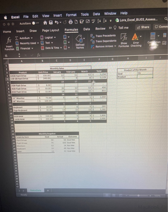
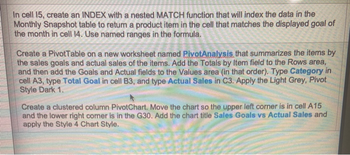
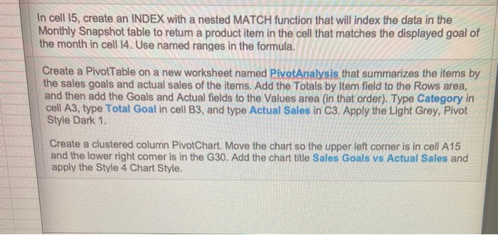
Excel File Edit View Insert Format Tools Data Window Help AutoSave SUODEON + + + Lora_Excel_BUO3 Assess... al Home Insert Draw Page Layout Formulas Data Review Tell me Share Comm Logical e Trace Precedents Recently Used Text Pg Trace Dependents Insert Defined Show Error Calon Function Financial Date & Time Names FRemove Arrows Formulas Checking OORS fx Autosum 15 H 1 D E Total Product 64GB Hard Drive 5 128GB Hard Drive Product of the Month Goal 75 Product 7 2GB Flash Drive B 4GB Flash Drive 9 SGB Flash Drive 10 11 15" Monitor 12 18" Monitor 13 14 Keyboard 15 Ergo Keyboard 16 17 BGB RAM 18 16GB RAM 19 20 Monthly Sales Unit Price January February March 150.00 12111255,250 3 78 55.229 19 17 20 $ 8.00 $ 10.00 20 12 13 5 450 S 15.00 18 20 19 5 855 32 32 s 75.00 5 455 1050 $ 100.00 5 5 $ 20.00 2 6 SS 260 $ 35.00 125 1260 15 17 17 s 150.00 4 5 1.100 5 200.00 2 3 SS 2.000 S Monthly Snapshot God 75 52 24 Totals by item 25 Hard Drives 26 Drwe 27 Motors 28 Keyboard 23 RAM 30 31 32 Actual Outco 56 Goal 102 Goal Mas 16 Met 49 Not Met 22 Goal Met 12 34 35 37 Salata Ready In cell 15, create an INDEX with a nested MATCH function that will index the data in the Monthly Snapshot table to return a product item in the cell that matches the displayed goal of the month in cell 14. Use named ranges in the formula. Create a PivotTable on a new worksheet named PivotAnalysis that summarizes the items by the sales goals and actual sales of the items. Add the Totals by Item field to the Rows area, and then add the Goals and Actual fields to the Values area (in that order). Type Category in cell A3, type Total Goal in cell B3, and type Actual Sales in C3. Apply the Light Grey, Pivot Style Dark 1. Create a clustered column PivotChart. Move the chart so the upper left corner is in cell A15 and the lower right comer is in the G30. Add the chart title Sales Goals vs Actual Sales and apply the Style 4 Chart Style. In cell 15, create an INDEX with a nested MATCH function that will index the data in the Monthly Snapshot table to retum a product item in the cell that matches the displayed goal of the month in cell 14. Use named ranges in the formula. Create a PivotTable on a new worksheet named PivotAnalysis that summarizes the items by the sales goals and actual sales of the items. Add the Totals by Item field to the Rows area, and then add the Goals and Actual fields to the Values area (in that order). Type Category in cell A3, type Total Goal in cell B3, and type Actual Sales in C3. Apply the Light Grey, Pivot Style Dark 1. Create a clustered column PivotChart. Move the chart so the upper left corner is in cell A15 and the lower right comer is in the G30. Add the chart title Sales Goals vs Actual Sales and apply the Style 4 Chart Style. Excel File Edit View Insert Format Tools Data Window Help AutoSave SUODEON + + + Lora_Excel_BUO3 Assess... al Home Insert Draw Page Layout Formulas Data Review Tell me Share Comm Logical e Trace Precedents Recently Used Text Pg Trace Dependents Insert Defined Show Error Calon Function Financial Date & Time Names FRemove Arrows Formulas Checking OORS fx Autosum 15 H 1 D E Total Product 64GB Hard Drive 5 128GB Hard Drive Product of the Month Goal 75 Product 7 2GB Flash Drive B 4GB Flash Drive 9 SGB Flash Drive 10 11 15" Monitor 12 18" Monitor 13 14 Keyboard 15 Ergo Keyboard 16 17 BGB RAM 18 16GB RAM 19 20 Monthly Sales Unit Price January February March 150.00 12111255,250 3 78 55.229 19 17 20 $ 8.00 $ 10.00 20 12 13 5 450 S 15.00 18 20 19 5 855 32 32 s 75.00 5 455 1050 $ 100.00 5 5 $ 20.00 2 6 SS 260 $ 35.00 125 1260 15 17 17 s 150.00 4 5 1.100 5 200.00 2 3 SS 2.000 S Monthly Snapshot God 75 52 24 Totals by item 25 Hard Drives 26 Drwe 27 Motors 28 Keyboard 23 RAM 30 31 32 Actual Outco 56 Goal 102 Goal Mas 16 Met 49 Not Met 22 Goal Met 12 34 35 37 Salata Ready In cell 15, create an INDEX with a nested MATCH function that will index the data in the Monthly Snapshot table to return a product item in the cell that matches the displayed goal of the month in cell 14. Use named ranges in the formula. Create a PivotTable on a new worksheet named PivotAnalysis that summarizes the items by the sales goals and actual sales of the items. Add the Totals by Item field to the Rows area, and then add the Goals and Actual fields to the Values area (in that order). Type Category in cell A3, type Total Goal in cell B3, and type Actual Sales in C3. Apply the Light Grey, Pivot Style Dark 1. Create a clustered column PivotChart. Move the chart so the upper left corner is in cell A15 and the lower right comer is in the G30. Add the chart title Sales Goals vs Actual Sales and apply the Style 4 Chart Style. In cell 15, create an INDEX with a nested MATCH function that will index the data in the Monthly Snapshot table to retum a product item in the cell that matches the displayed goal of the month in cell 14. Use named ranges in the formula. Create a PivotTable on a new worksheet named PivotAnalysis that summarizes the items by the sales goals and actual sales of the items. Add the Totals by Item field to the Rows area, and then add the Goals and Actual fields to the Values area (in that order). Type Category in cell A3, type Total Goal in cell B3, and type Actual Sales in C3. Apply the Light Grey, Pivot Style Dark 1. Create a clustered column PivotChart. Move the chart so the upper left corner is in cell A15 and the lower right comer is in the G30. Add the chart title Sales Goals vs Actual Sales and apply the Style 4 Chart Style