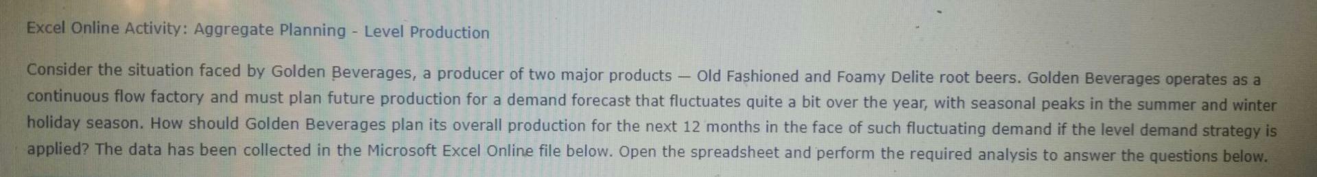
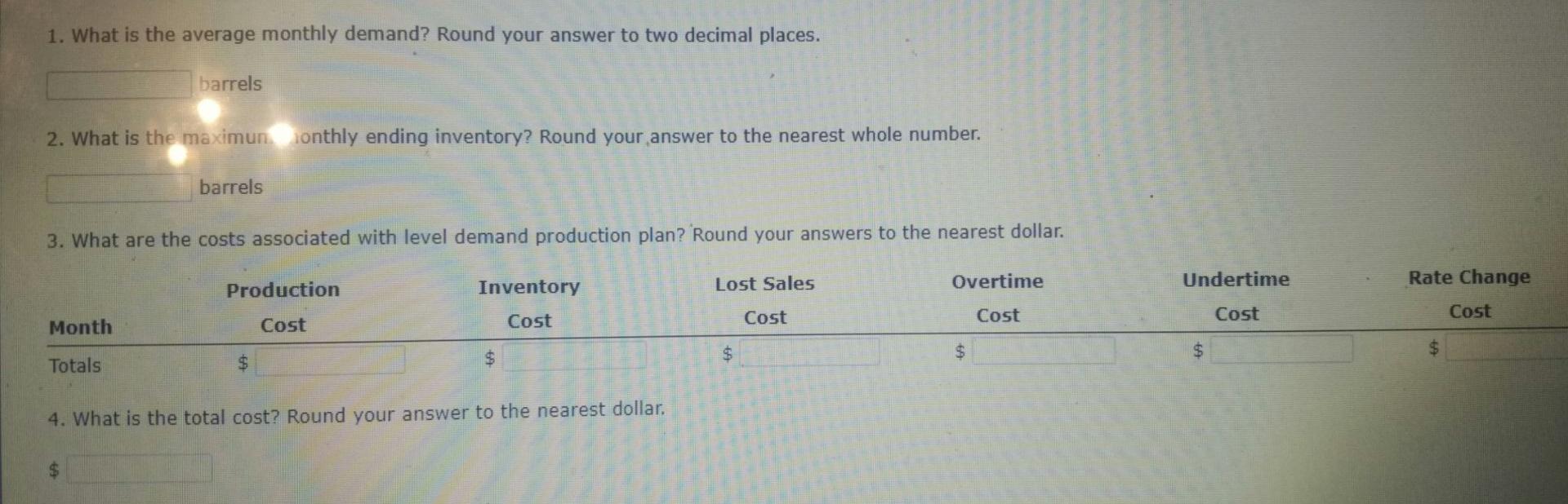
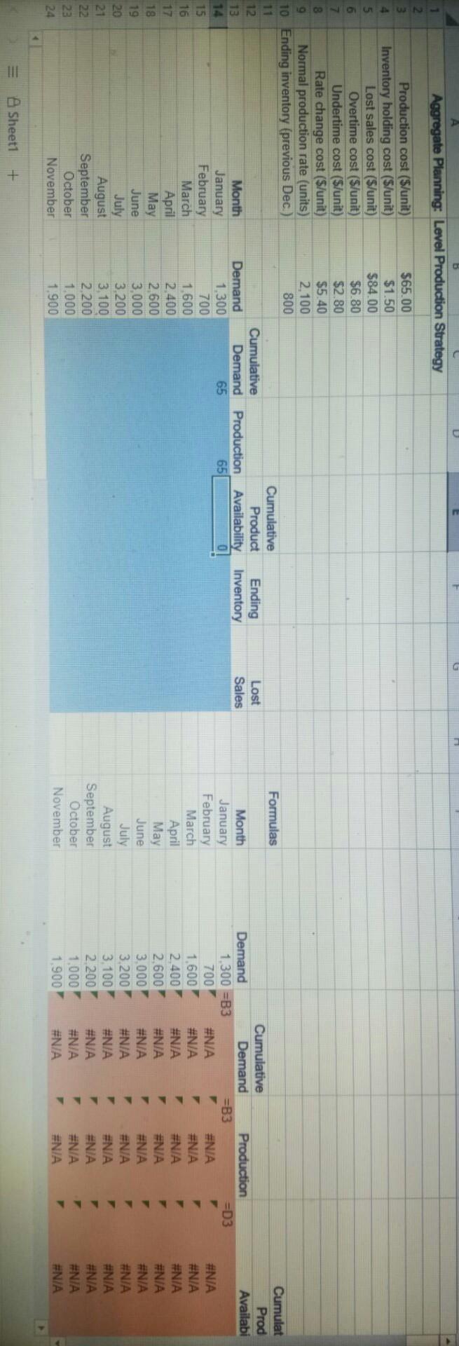
Excel Online Activity: Aggregate Planning - Level Production Consider the situation faced by Golden Beverages, a producer of two major products - Old Fashioned and Foamy Delite root beers. Golden Beverages operates as a continuous flow factory and must plan future production for a demand forecast that fluctuates quite a bit over the year, with seasonal peaks in the summer and winter holiday season. How should Golden Beverages plan its overall production for the next 12 months in the face of such fluctuating demand if the level demand strategy is applied? The data has been collected in the Microsoft Excel Online file below. Open the spreadsheet and perform the required analysis to answer the questions below. 1. What is the average monthly demand? Round your answer to two decimal places. barrels 2. What is the maximun ionthly ending inventory? Round your answer to the nearest whole number. barrels 3. What are the costs associated with level demand production plan? Round your answers to the nearest dollar. Overtime Undertime Lost Sales Production Inventory Rate Change Cost Cost Cost Cost Cost Month Cost $ $ $ $ Totals $ $ 4. What is the total cost? Round your answer to the nearest dollar. $ Formulas 1 Aggregate Planning: Level Production Strategy 2. 3 Production cost (5/unit) $65.00 4. Inventory holding cost ($/unit) $1.50 5 Lost sales cost ($/unit) $84.00 6 Overtime cost ($/unit) $6.80 7 Undertime cost ($/unit) $2.80 8 Rate change cost ($/unit) $5.40 9 Normal production rate (units) 2.100 10 Ending inventory (previous Dec.) 800 11 Cumulative 12 Cumulative Product Ending 13 Month Demand Demand Production Availability Inventory 14 January 1.300 65 65 15 February 700 16 March 1.600 17 April 2.400 18 May 2.600 19 June 3.000 20 July 3.200 21 August 3.100 22 September 2.200 23 October 1.000 24 November 1.900 Lost Sales Cumulat Prod Availabi Month January February March April May June July August September October November Cumulative Demand Demand Production 1.300 =B3 =B3 =D3 700 #N/A #NIA 1.600 #N/A #N/A 2.400 #N/A #N/A 2.600 #N/A #N/A 3.000 #N/A 3.200 #NIA #N/A 3.100 #N/A #N/A 2.200 #N/A ENIA 1.000 #N/A #N/A 1.900 #N/A #N/A #NIA #N/A #N/A #N/A #N/A #N/A #N/A #N/A #N/A #N/A #N/A 4 III A Sheet1 + Excel Online Activity: Aggregate Planning - Level Production Consider the situation faced by Golden Beverages, a producer of two major products - Old Fashioned and Foamy Delite root beers. Golden Beverages operates as a continuous flow factory and must plan future production for a demand forecast that fluctuates quite a bit over the year, with seasonal peaks in the summer and winter holiday season. How should Golden Beverages plan its overall production for the next 12 months in the face of such fluctuating demand if the level demand strategy is applied? The data has been collected in the Microsoft Excel Online file below. Open the spreadsheet and perform the required analysis to answer the questions below. 1. What is the average monthly demand? Round your answer to two decimal places. barrels 2. What is the maximun ionthly ending inventory? Round your answer to the nearest whole number. barrels 3. What are the costs associated with level demand production plan? Round your answers to the nearest dollar. Overtime Undertime Lost Sales Production Inventory Rate Change Cost Cost Cost Cost Cost Month Cost $ $ $ $ Totals $ $ 4. What is the total cost? Round your answer to the nearest dollar. $ Formulas 1 Aggregate Planning: Level Production Strategy 2. 3 Production cost (5/unit) $65.00 4. Inventory holding cost ($/unit) $1.50 5 Lost sales cost ($/unit) $84.00 6 Overtime cost ($/unit) $6.80 7 Undertime cost ($/unit) $2.80 8 Rate change cost ($/unit) $5.40 9 Normal production rate (units) 2.100 10 Ending inventory (previous Dec.) 800 11 Cumulative 12 Cumulative Product Ending 13 Month Demand Demand Production Availability Inventory 14 January 1.300 65 65 15 February 700 16 March 1.600 17 April 2.400 18 May 2.600 19 June 3.000 20 July 3.200 21 August 3.100 22 September 2.200 23 October 1.000 24 November 1.900 Lost Sales Cumulat Prod Availabi Month January February March April May June July August September October November Cumulative Demand Demand Production 1.300 =B3 =B3 =D3 700 #N/A #NIA 1.600 #N/A #N/A 2.400 #N/A #N/A 2.600 #N/A #N/A 3.000 #N/A 3.200 #NIA #N/A 3.100 #N/A #N/A 2.200 #N/A ENIA 1.000 #N/A #N/A 1.900 #N/A #N/A #NIA #N/A #N/A #N/A #N/A #N/A #N/A #N/A #N/A #N/A #N/A 4 III A Sheet1 +