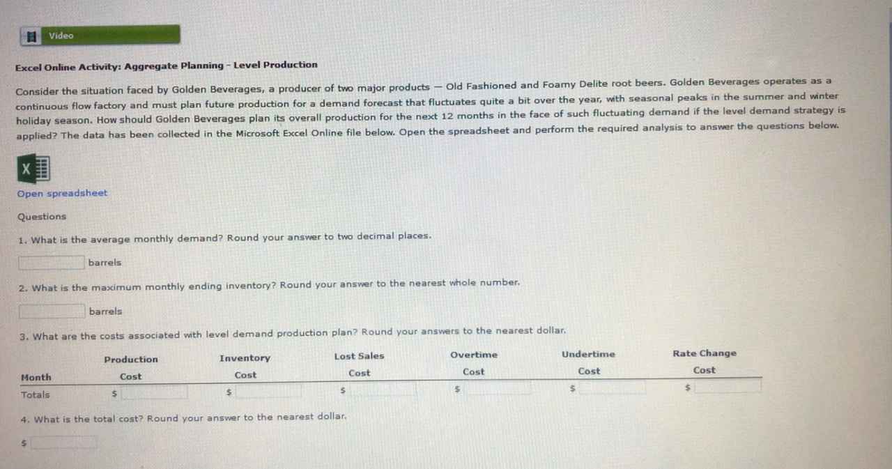
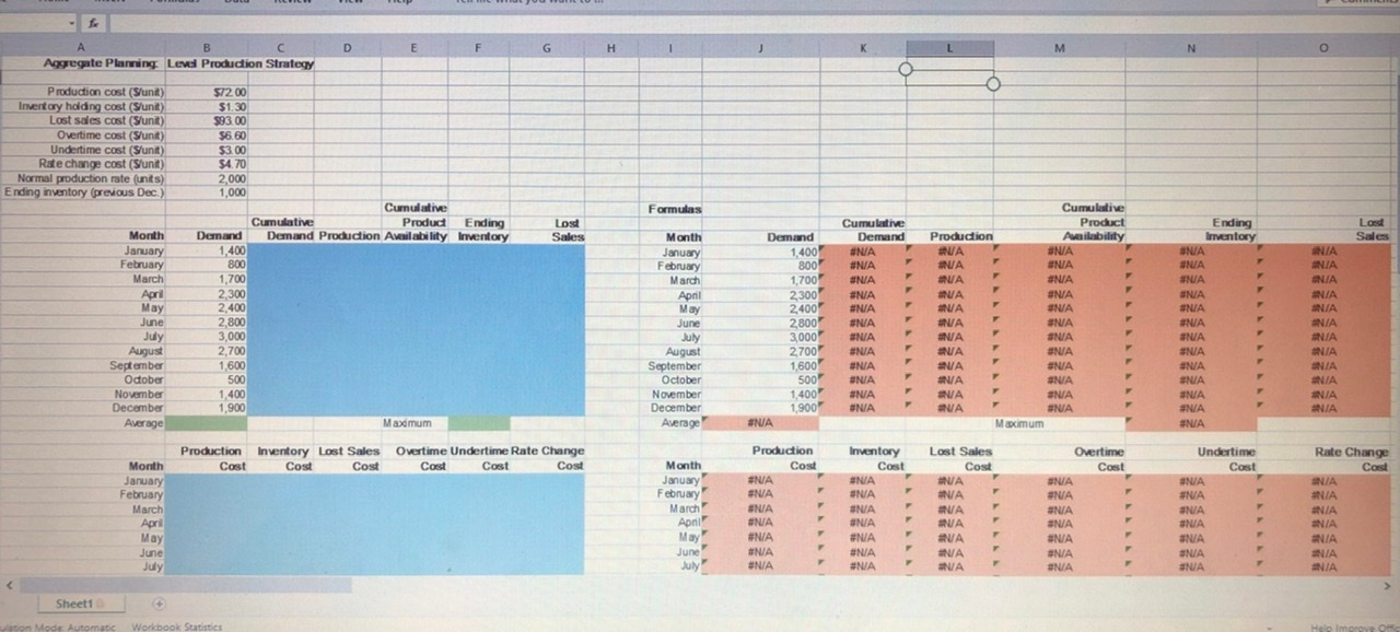
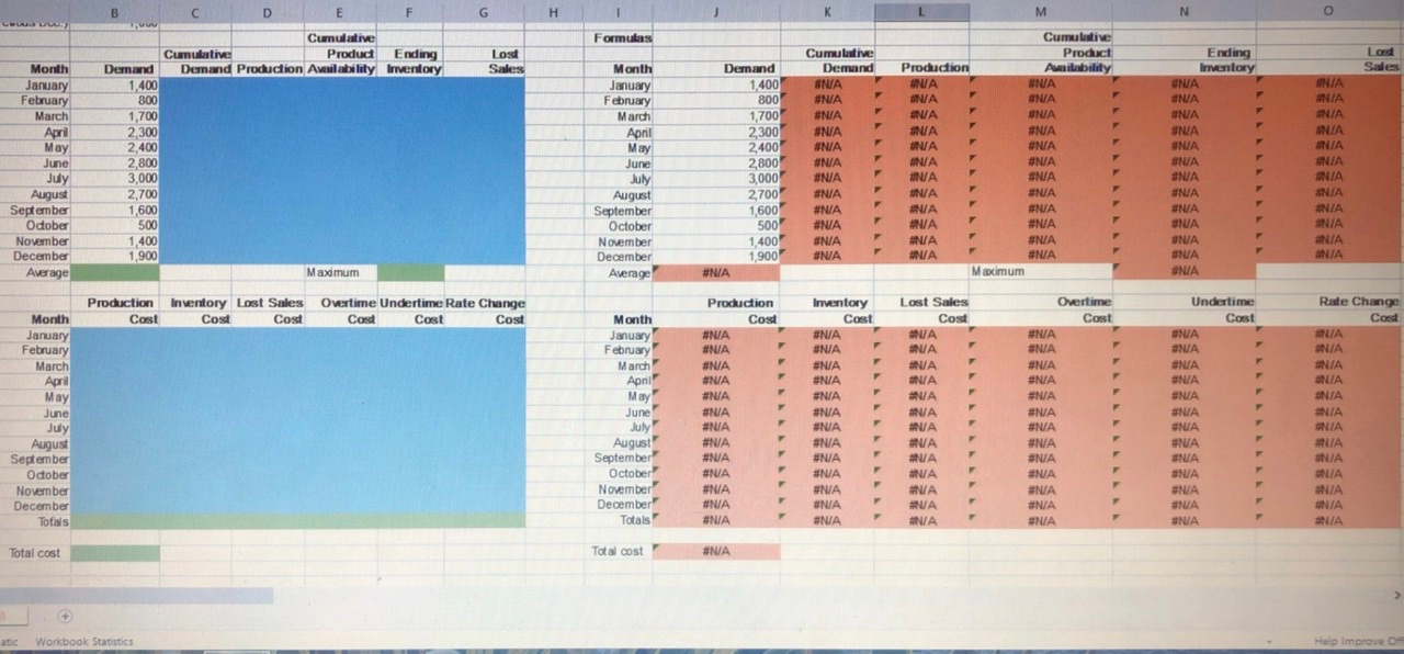
Video Excel Online Activity: Aggregate Planning - Level Production Consider the situation faced by Golden Beverages, a producer of two major products - Old Fashioned and Foamy Delite root beers. Golden Beverages operates as a continuous flow factory and must plan future production for a demand forecast that fluctuates quite a bit over the year, with seasonal peaks in the summer and winter holiday season. How should Golden Beverages plan its overall production for the next 12 months in the face of such fluctuating demand if the level demand strategy is applied? The data has been collected in the Microsoft Excel Online file below. Open the spreadsheet and perform the required analysis to answer the questions below. X Open spreadsheet Questions 1. What is the average monthly demand? Round your answer to two decimal places. barrels 2. What is the maximum monthly ending inventory? Round your answer to the nearest whole number. barrels 3. What are the costs associated with level demand production plan? Round your answers to the nearest dollar. Lost Sales Inventory Cost Overtime Cost Undertime Cost Production Cost $ Rate Change Cost Month Cost $ $ $ 5 Totals 4. What is the total cost? Round your answer to the nearest dollar, D E F H 1 M N A B Aggregate Planning Level Production Strategy Production cost (Sunit) Inventory holding cost (S/unit) Lost sales cost (S/unit) Overtime cost (S/unit) Undertime cost (S/unit) Rate change cost (S/unit) Normal production rate (unts) Ending inventory (previous Dec Formulas Los Sales Lord Sales Month January February March April May June July August September Odober November December Average 57200 $1.30 $93.00 $6.60 $3.00 $4.70 2,000 1,000 Cumulative Cumulative Product Ending Demand Demand Production Availability Inventory 1,400 800 1,700 2,300 2,400 2,800 3,000 2,700 1,600 500 1,400 1,900 Maximum Month January February March April May June July August September October November December Average Demand 1.400 800 1.700 2300 2400 2800 3,000 Cumulative Demand #N/A #N/A #N/A #N/A #N/A #N/A NA #NIA F SNIA ENIA SNA UNIA Cumulative Product Production Availability RUA #N/A WA NIA MA SNIA WA SN/A WA #NA NA F F NA ANIA SNIA ANA SNA NA SNA F N/A SNA NA ANA ANIA SNA Macimum Ending Inventory #N/A #NA #NIA #NIA ANIA NA NA #NA N/A ENIA #NA #N/A #N/A NIA ANIA ENIA ANIA ANIA N/A INIA NIA NIA ANIA NIA ANIA 2700 1,600 500 1.400 1.900 #NA Inventory Production Inventory Lost Sales Cost Cost Cost Overtime Undertime Rate Change Cost Corst Cost Month January February March Apri May Month January February March April Production Cost SNA SNIA #NA #NA #N/A #NIA #N/A Cost SNA NA N/A NA #N/A #N/A #NA Lost Sales Cost NA F NA WA WA NA NA NA Overtime Cost NA SNA SNIA SNA NA N/A NIA Undertime Cost NA #N/A #N/A #NA NIA SNIA #NA Rate Change Cost NIA ANIA INIA ANIA ANIA NIA ANIA May June June July July Sheet1 15 Mode Automatic Workbook Statistics Helo In B D E F G H K M N LISUUS Formulas Los Sales Lord Sales Month January February Cumulative Cumulative Product Ending Demand Demand Production Awailability Inventory 1,400 800 1,700 2,300 2,400 2.800 3.000 2,700 1,600 500 1,400 1,900 Maximum March April May June July August September Odober November December Average Month January February March April May June July August September October November December Average Cumulative Demand #NA #N/A F #N/A #N/A #N/A #N/A #N/A #N/A #N/A #N/A #N/A #N/A Demand 1,400 800 1,700 2300 2400 2800 3,000 2700 1,600 500 1,400 1,900 #N/A ANIA ANIA ANIA ANIA ANIA ANIA Cumulative Product Production Anilability ANIA ONA ANA #N/A ANIA # #NIA N/A #N/A UNA #NA ANIA #N/A UNA #N/A #N/A #N/A #N/A #NA #N/A #N/A ANIA #N/A N/A #N/A Maximum Ending Inventory #N/A ONIA #N/A #NA #NA ENIA #N/A NA ENA #N/A UNA NA #N/A NA INIA UNIA NIA ANIA WNIA Production Inventory Lost Sales Cost Cost Cost Overtime Undertime Rate Change Cost Cost Cost Month January February March April May June July August September Odober November December Totals Month January February March Apni May June July August September October November December Totals Production Cost #N/A #N/A / #N/A #N/A #N/A #N/A #NIA #N/A #N/A #N/A #N/A #N/A #N/A Inventory Cost #N/A #N/A #N/A #N/A #N/A #N/A #N/A #NA #NA #NIA #N/A #N/A #N/A F Lost Sales Cos NA ANA NA INA #N/A F INIA F NA N/A ANA NIA N/A ANA ANIA Overtime Cost #N/A #N/A #N/A #N/A #N/A F #N/A #N/A #N/A #N/A #N/A #N/A #N/A #N/A Undertime Cost #N/A #N/A ENJA SNIA ENA NA NA #N/A #NIA SNIA #N/A N/A NA Rate Change Cord ANIA NA NIA #N/A ANIA NIA NIA ANIA ANIA NIA NIA NIA NIA Total cost Total cost #N/A Workbook Statistics Help Improve o Video Excel Online Activity: Aggregate Planning - Level Production Consider the situation faced by Golden Beverages, a producer of two major products - Old Fashioned and Foamy Delite root beers. Golden Beverages operates as a continuous flow factory and must plan future production for a demand forecast that fluctuates quite a bit over the year, with seasonal peaks in the summer and winter holiday season. How should Golden Beverages plan its overall production for the next 12 months in the face of such fluctuating demand if the level demand strategy is applied? The data has been collected in the Microsoft Excel Online file below. Open the spreadsheet and perform the required analysis to answer the questions below. X Open spreadsheet Questions 1. What is the average monthly demand? Round your answer to two decimal places. barrels 2. What is the maximum monthly ending inventory? Round your answer to the nearest whole number. barrels 3. What are the costs associated with level demand production plan? Round your answers to the nearest dollar. Lost Sales Inventory Cost Overtime Cost Undertime Cost Production Cost $ Rate Change Cost Month Cost $ $ $ 5 Totals 4. What is the total cost? Round your answer to the nearest dollar, D E F H 1 M N A B Aggregate Planning Level Production Strategy Production cost (Sunit) Inventory holding cost (S/unit) Lost sales cost (S/unit) Overtime cost (S/unit) Undertime cost (S/unit) Rate change cost (S/unit) Normal production rate (unts) Ending inventory (previous Dec Formulas Los Sales Lord Sales Month January February March April May June July August September Odober November December Average 57200 $1.30 $93.00 $6.60 $3.00 $4.70 2,000 1,000 Cumulative Cumulative Product Ending Demand Demand Production Availability Inventory 1,400 800 1,700 2,300 2,400 2,800 3,000 2,700 1,600 500 1,400 1,900 Maximum Month January February March April May June July August September October November December Average Demand 1.400 800 1.700 2300 2400 2800 3,000 Cumulative Demand #N/A #N/A #N/A #N/A #N/A #N/A NA #NIA F SNIA ENIA SNA UNIA Cumulative Product Production Availability RUA #N/A WA NIA MA SNIA WA SN/A WA #NA NA F F NA ANIA SNIA ANA SNA NA SNA F N/A SNA NA ANA ANIA SNA Macimum Ending Inventory #N/A #NA #NIA #NIA ANIA NA NA #NA N/A ENIA #NA #N/A #N/A NIA ANIA ENIA ANIA ANIA N/A INIA NIA NIA ANIA NIA ANIA 2700 1,600 500 1.400 1.900 #NA Inventory Production Inventory Lost Sales Cost Cost Cost Overtime Undertime Rate Change Cost Corst Cost Month January February March Apri May Month January February March April Production Cost SNA SNIA #NA #NA #N/A #NIA #N/A Cost SNA NA N/A NA #N/A #N/A #NA Lost Sales Cost NA F NA WA WA NA NA NA Overtime Cost NA SNA SNIA SNA NA N/A NIA Undertime Cost NA #N/A #N/A #NA NIA SNIA #NA Rate Change Cost NIA ANIA INIA ANIA ANIA NIA ANIA May June June July July Sheet1 15 Mode Automatic Workbook Statistics Helo In B D E F G H K M N LISUUS Formulas Los Sales Lord Sales Month January February Cumulative Cumulative Product Ending Demand Demand Production Awailability Inventory 1,400 800 1,700 2,300 2,400 2.800 3.000 2,700 1,600 500 1,400 1,900 Maximum March April May June July August September Odober November December Average Month January February March April May June July August September October November December Average Cumulative Demand #NA #N/A F #N/A #N/A #N/A #N/A #N/A #N/A #N/A #N/A #N/A #N/A Demand 1,400 800 1,700 2300 2400 2800 3,000 2700 1,600 500 1,400 1,900 #N/A ANIA ANIA ANIA ANIA ANIA ANIA Cumulative Product Production Anilability ANIA ONA ANA #N/A ANIA # #NIA N/A #N/A UNA #NA ANIA #N/A UNA #N/A #N/A #N/A #N/A #NA #N/A #N/A ANIA #N/A N/A #N/A Maximum Ending Inventory #N/A ONIA #N/A #NA #NA ENIA #N/A NA ENA #N/A UNA NA #N/A NA INIA UNIA NIA ANIA WNIA Production Inventory Lost Sales Cost Cost Cost Overtime Undertime Rate Change Cost Cost Cost Month January February March April May June July August September Odober November December Totals Month January February March Apni May June July August September October November December Totals Production Cost #N/A #N/A / #N/A #N/A #N/A #N/A #NIA #N/A #N/A #N/A #N/A #N/A #N/A Inventory Cost #N/A #N/A #N/A #N/A #N/A #N/A #N/A #NA #NA #NIA #N/A #N/A #N/A F Lost Sales Cos NA ANA NA INA #N/A F INIA F NA N/A ANA NIA N/A ANA ANIA Overtime Cost #N/A #N/A #N/A #N/A #N/A F #N/A #N/A #N/A #N/A #N/A #N/A #N/A #N/A Undertime Cost #N/A #N/A ENJA SNIA ENA NA NA #N/A #NIA SNIA #N/A N/A NA Rate Change Cord ANIA NA NIA #N/A ANIA NIA NIA ANIA ANIA NIA NIA NIA NIA Total cost Total cost #N/A Workbook Statistics Help Improve o