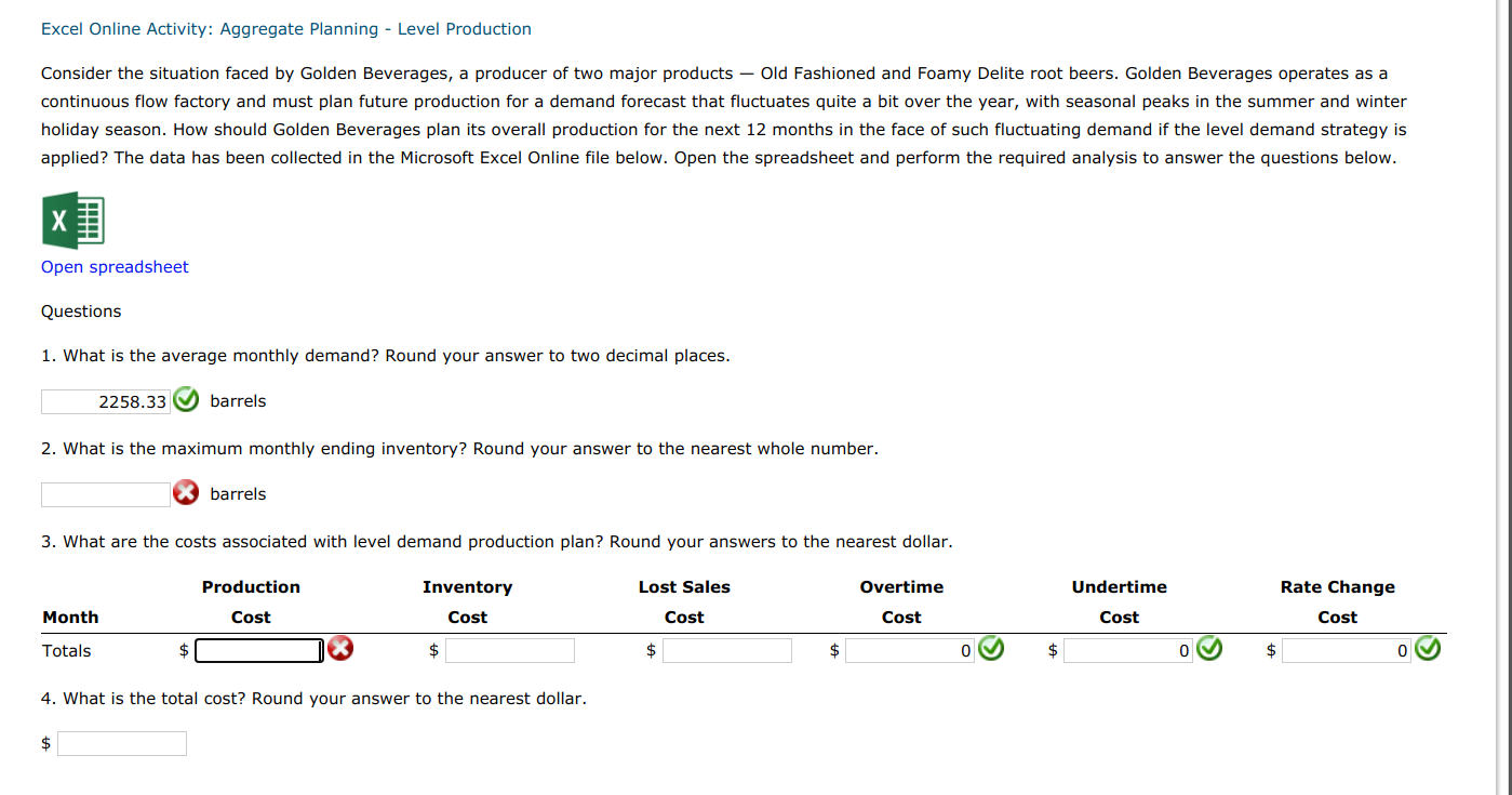
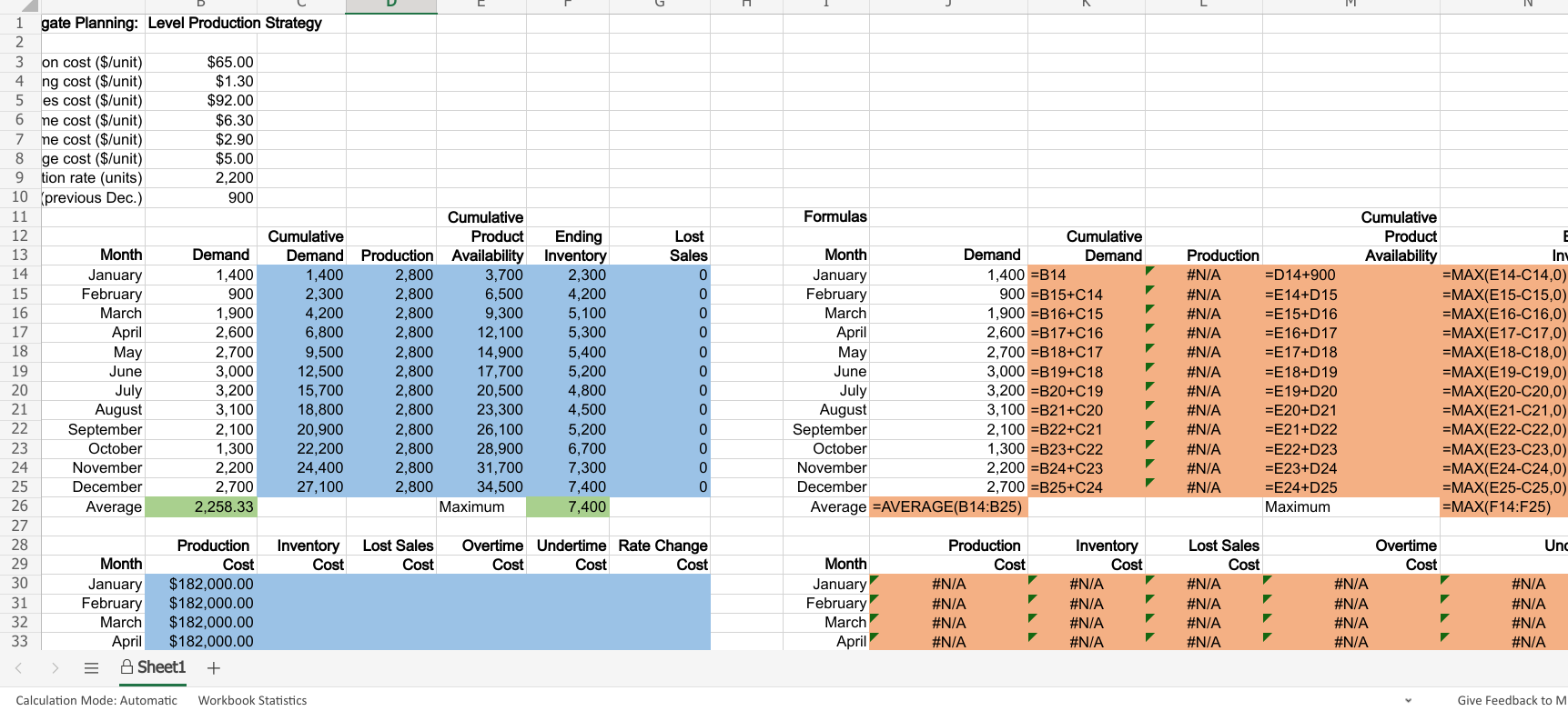
Excel Online Activity: Aggregate Planning - Level Production Consider the situation faced by Golden Beverages, a producer of two major products Old Fashioned and Foamy Delite root beers. Golden Beverages operates as a continuous flow factory and must plan future production for a demand forecast that fluctuates quite a bit over the year, with seasonal peaks in the summer and winter holiday season. How should Golden Beverages plan its overall production for the next 12 months in the face of such fluctuating demand if the level demand strategy is applied? The data has been collected in the Microsoft Excel Online file below. Open the spreadsheet and perform the required analysis to answer the questions below. X Open spreadsheet Questions 1. What is the average monthly demand? Round your answer to two decimal places. 2258.33 barrels 2. What is the maximum monthly ending inventory? Round your answer to the nearest whole number. barrels 3. What are the costs associated with level demand production plan? Round your answers to the nearest dollar. Production Lost Sales Overtime Undertime Rate Change Inventory Cost Month Cost Cost Cost Cost Cost Totals $ $ $ 0 $ 0 0 4. What is the total cost? Round your answer to the nearest dollar. $ C 1 gate Planning: Level Production Strategy 2 3 on cost ($/unit) $65.00 4 ng cost ($/unit) $1.30 5 es cost ($/unit) $92.00 6 ne cost ($/unit) $6.30 7 ne cost ($/unit) $2.90 8 ge cost ($/unit) $5.00 9 tion rate (units) 2,200 10 previous Dec.) 900 11 Cumulative 12 Cumulative Product Ending Lost 13 Month Demand Demand Production Availability Inventory Sales 14 January 1,400 1,400 2,800 3,700 2,300 0 15 February 900 2,300 2,800 6,500 4,200 0 16 March 1,900 4,200 2,800 9,300 5,100 0 17 April 2,600 6,800 2,800 12,100 5,300 0 18 May 2,700 9,500 2,800 14,900 5,400 0 19 June 3,000 12,500 2,800 17,700 5,200 0 20 July 3,200 15,700 2,800 20,500 4,800 0 21 August 3,100 18,800 2,800 23,300 4,500 0 22 September 2,100 20,900 2,800 26,100 5,200 0 23 October 1,300 22,200 2,800 28,900 6,700 24 November 2,200 24,400 2,800 31.700 7,300 0 25 December 2,700 27,100 2,800 34.500 7,400 0 26 Average 2,258.33 Maximum 7,400 27 28 Production Inventory Lost Sales Overtime Undertime Rate Change 29 Month Cost Cost Cost Cost Cost Cost 30 January $182,000.00 31 February $182,000.00 32 March $182,000.00 33 April $182,000.00 = A Sheet1 + Formulas Cumulative Month Demand Demand January 1,400 =B14 February 900 =B15+C14 March 1,900 =B16+C15 April 2,600 =B17+C16 May 2,700 =B18+C17 June 3,000 =B19+C18 July 3,200 =B20+C19 August 3,100 =B21+C20 September 2,100 =B22+C21 October 1,300 =B23+C22 November 2,200 =B24+C23 December 2,700 =B25+C24 Average =AVERAGE(B14:B25) Production #N/A D14+900 #N/A =E14+D15 #N/A E15+D16 #N/A =E16+D17 #N/A =E17+D18 #N/A =E18+D19 #N/A =E19+D20 #N/A =E20+D21 #N/A =E21+D22 #N/A =E22+D23 #N/A =E23+D24 #N/A =E24+D25 Maximum Cumulative Product E Availability Iny =MAX(E14-C14,0) =MAX(E15-C15,0) =MAX(E16-C16,0) =MAX(E17-C17,0) =MAX(E18-C18,0) =MAX(E19-C19,0) =MAX(E20-C20,0) =MAX(E21-C21,0) =MAX(E22-C22,0) =MAX(E23-C23,0) =MAX(E24-C24,0) =MAX(E25-C25,0) =MAX(F14:F25) Unc Month January February March April Production Cost #N/A #N/A #N/A #N/A Inventory Cost #N/A #N/A Lost Sales Cost #N/A #N/A #N/A #N/A Overtime Cost #N/A #N/A #N/A #N/A #N/A #N/A #N/A #N/A #N/A #N/A Calculation Mode: Automatic Workbook Statistics Give Feedback to M