Question: EXCEL - Please help! 9. Change the summary function to Average for the data in the Values area and apply the Number number format with

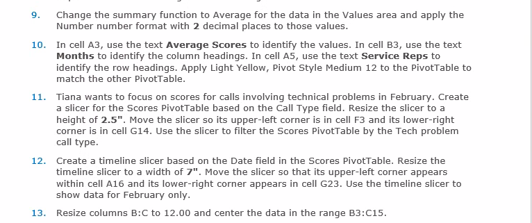
EXCEL - Please help! 9. Change the summary function to Average for the data in the Values area and apply the Number number format EXCEL - Please help!

9. Change the summary function to Average for the data in the Values area and apply the Number number format with 2 decimal places to those values. 10. In cell A3, use the text Average Scores to identify the values. In cell B3, use the text Months to identify the column headings. In cell A5, use the text Service Reps to identify the row headings. Apply Light Yellow, Pivot Style Medium 12 to the PivotTable to match the other PivotTable. 11. Tiana wants to focus on scores for calls involving technical problems in February. Create a slicer for the Scores PivotTable based on the Call Type field. Resize the slicer to a height of 2.5. Move the slicer so its upper-left corner is in cell F3 and its lower-right corner is in cell G14. Use the slicer to filter the Scores PivotTable by the Tech problem call type. 12. Create a timeline slicer based on the Date field in the Scores PivotTable. Resize the timeline slicer to a width of 7". Move the slicer so that its upper-left corner appears within cell A16 and its lower-right corner appears in cell G23. Use the timeline slicer to show data for February only. 13. Resize columns B:C to 12.00 and center the data in the range B3:C15. 9. Change the summary function to Average for the data in the Values area and apply the Number number format with 2 decimal places to those values. 10. In cell A3, use the text Average Scores to identify the values. In cell B3, use the text Months to identify the column headings. In cell A5, use the text Service Reps to identify the row headings. Apply Light Yellow, Pivot Style Medium 12 to the PivotTable to match the other PivotTable. 11. Tiana wants to focus on scores for calls involving technical problems in February. Create a slicer for the Scores PivotTable based on the Call Type field. Resize the slicer to a height of 2.5. Move the slicer so its upper-left corner is in cell F3 and its lower-right corner is in cell G14. Use the slicer to filter the Scores PivotTable by the Tech problem call type. 12. Create a timeline slicer based on the Date field in the Scores PivotTable. Resize the timeline slicer to a width of 7". Move the slicer so that its upper-left corner appears within cell A16 and its lower-right corner appears in cell G23. Use the timeline slicer to show data for February only. 13. Resize columns B:C to 12.00 and center the data in the range B3:C15

Step by Step Solution

There are 3 Steps involved in it

1 Expert Approved Answer

Step: 1 Unlock blur-text-image

Question Has Been Solved by an Expert!

Get step-by-step solutions from verified subject matter experts

Step: 2 Unlock

Step: 3 Unlock

Students Have Also Explored These Related Accounting Questions!

48 49 50 51 52 Add values to a PivotTable. 9. Change the summary function to Average for the data in the Values area and apply the Number number format with 2 decimal places to those values. X...

1. Tiana Morales is the director of the customer call center for Pierce Software. For the past three months, she has been keeping track of the support calls the center receives, and asks for your...

Change the summary function to Average for the data in the Values area and apply the Number number format with 2 decimal places to those values. In cell A 3 , use the text Average Scores to identify...

This is an excel assignment, I don't have time to do it, so i need help to do it FIN 310 Excel Assignment #3 Due Friday, 6/10 by 5 pm READ ALL INSTRUCTIONS BEFORE BEGINNING Save your file as...

Please Leave clear step by step instructions with listed cells and formulas. Thank you! Barbara received some additional data from the distributor that she needs to analyze and give to the marketing...

Hide Assignment Information Instructions HMGT 4 0 0 Research and Data Analysis in Health Care - Exercise Dataset:HMGTHOSP.csv ( Please download dataset from the class. ) Required program: for all...

The instructions step by step are the questions Step Instructions Points Possible 0 N 2 4 3 Start Excel. Download and open the file named Exp19_Excel_Ch05_CapAssessment_Travel.xlsx Grader has...

Project Description: You are the manager of an information technology (IT) team. Your employees go to training workshops and national conferences to keep up-to-date in the field. You created a list...

Points Possible Instructions 13 Change the name for the Expenses column to Totals and format the field with Accounting number format. 6 Insert a calculated field to subtract 2659.72 from the Expense...

Flextech Inc. is considering a project that will require new equipment costing $150,000. It will replace old equipment with a book value of $35,000 that can be sold on the secondhand market for...

Describe managerial derailment and provide three examples

Mutual Funds invest funds in a portfolio of financial instruments True False

Which of the following are problems with identifying users of ABC? Multiple select question. ABC means different things to different organizations. Organizations will announce the discontinuance of...

Jason Ochi purchased an in-home gym during the Anniversary Sale at Workout City. During the Anniversary Sale, a special promotion was running that allowed Jason to qualify for 0 percent interest for...

Name and describe the nature of the three common informal report types described in this chapter. (Objective 2)

Kent Fulsom has been a credit customer of Thurman Furniture Store for eight years. He is a good customer but periodically fails to make payments on his account. He is currently four months past due...