EXECEL WORK. can anyone help question 3-29. Please if you can't do everything dont start

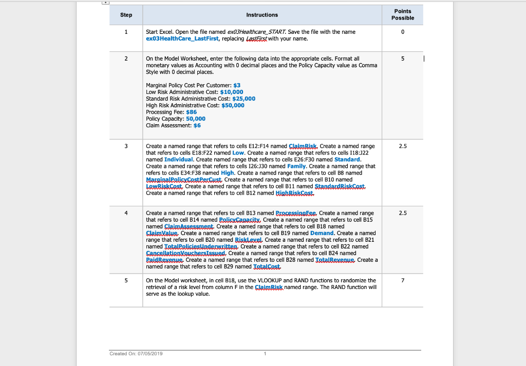
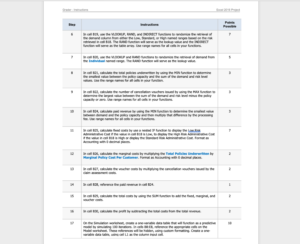
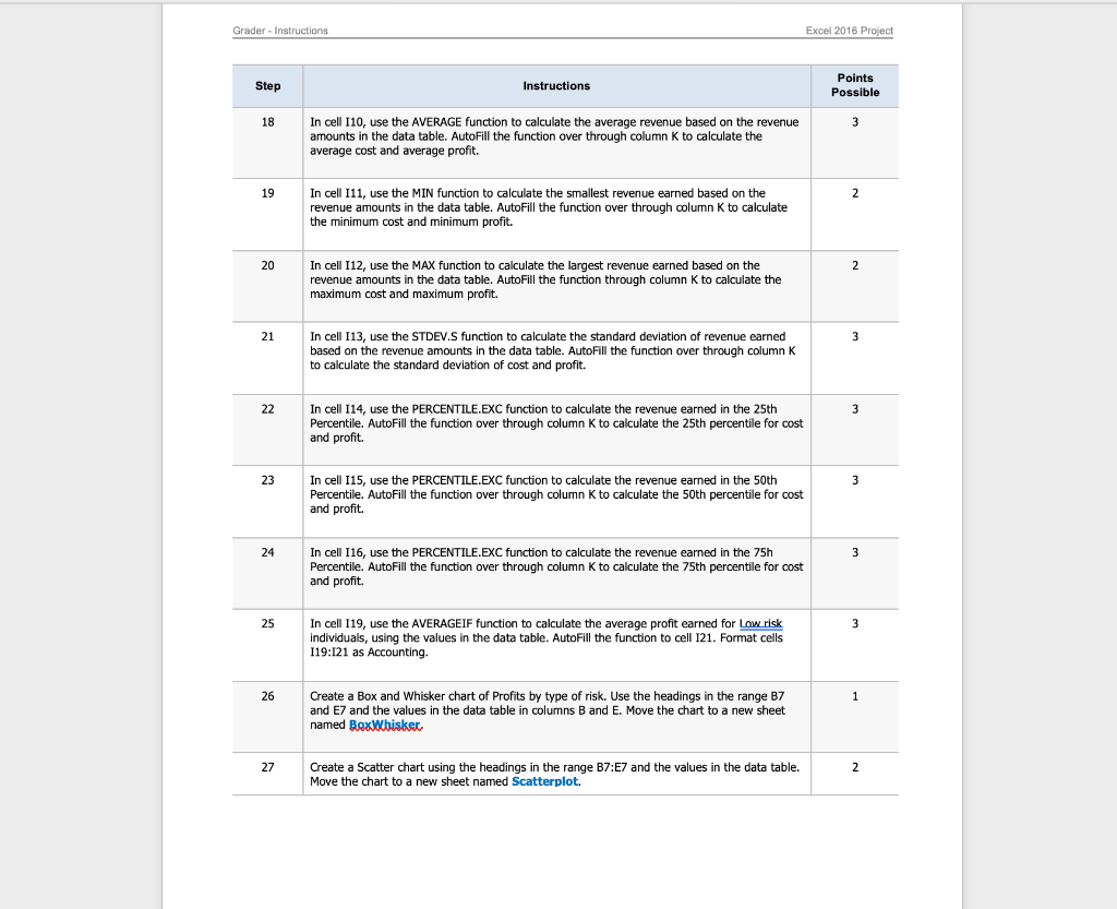
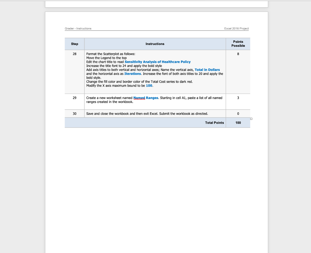
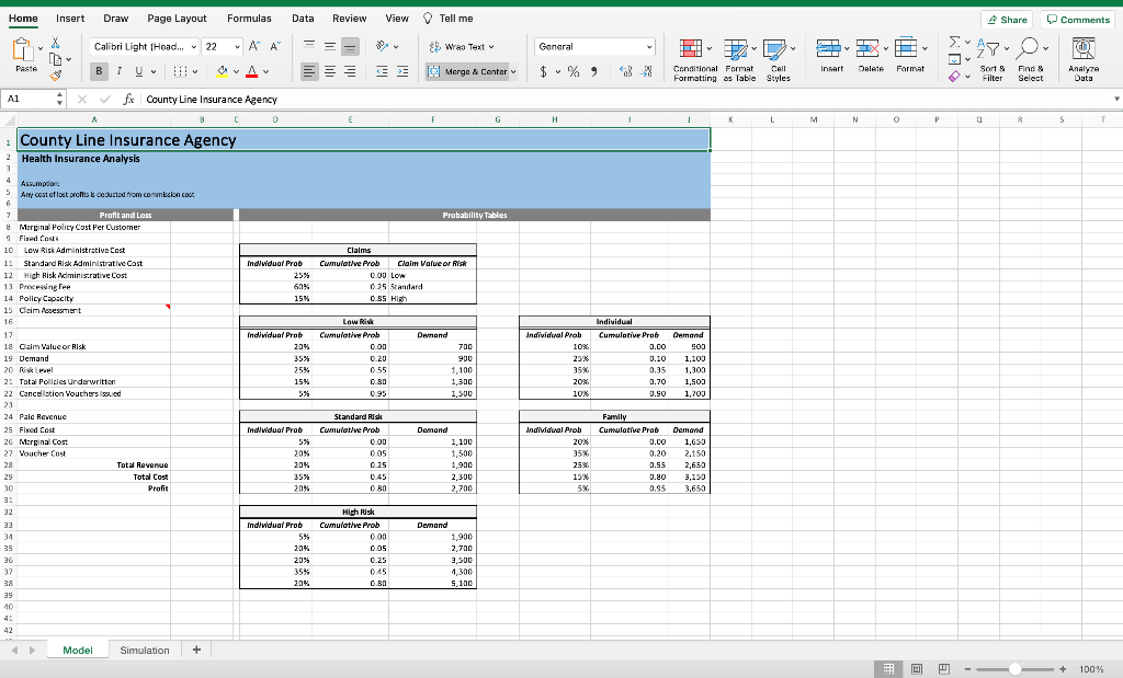
Step Instructions Points Possible 1 0 Start Excel. Open the file named exO3Healthcare_START. Save the file with the name exO3Health Care_LastFirst, replacing LastFirst with your name. 2 5 1 On the Model Worksheet, enter the following data into the appropriate cells. Format all monetary values as Accounting with 0 decimal places and the Policy Capacity value as comma Style with O decimal places. Marginal Policy Cost Per Customer: $3 Low Risk Administrative Cost: $10,000 Standard Risk Administrative Cost: $25,000 High Risk Administrative Cost: $50,000 Processing Fee: $86 Policy Capacity: 50,000 Claim Assessment: $6 3 2.5 Create a named range that refers to cells E12:F14 named Claim Risk, Create a named range that refers to cells E18:F22 named Low. Create a named range that refers to cells 118:122 named Individual. Create named range that refers to cells E26:F30 named Standard. Create a named range that refers to cells 126:130 named Family. Create a named range that refers to cells E34:F38 named High. Create a named range that refers to cell B8 named Marginal PolicyCast Per Cust. Create a named range that refers to cell B10 named LowBisk Cast, Create a named range that refers to cell B11 named Standard Risk Cost Create a named range that refers to cell B12 named High Riskcost 4 2.5 Create a named range that refers to cell B13 named ProcessingFee. Create a named range that refers to cell B14 named PelisxCapacity, Create a named range that refers to cell B15 named Claim Assessment. Create a named range that refers to cell B18 named Claim Value. Create a named range that refers to cell B19 named Demand. Create a named range that refers to cell B20 named Risklexel. Create a named range that refers to cell B21 named Tatal policies Underwritten. Create a named range that refers to cell B22 named Cancellation VouchersIssued. Create a named range that refers to cell B24 named Paid Revenue. Create a named range that refers to cell B28 named Total Revenue Create a named range that refers to cell B29 named Tatal cost 5 7 On the Model worksheet, in cell B18, use the VLOOKUP and RAND functions to randomize the retrieval of a risk level from column F in the Claim Risk named range. The RAND function will serve as the lookup value. Created On: 07/05/2019 Grader - Instructions Excel 2016 Project Step Instructions Points Possible 6 7 In cell B19, use the VLOOKUP, RAND, and INDIRECT functions to randomize the retrieval of the demand column from either the Low, Standard, or High named ranges based on the risk retrieved in cell B18. The RAND function will serve as the lookup value and the INDIRECT function will serve as the table array. Use range names for all cells in your functions. 7 5 In cell B20, use the VLOOKUP and RAND functions to randomize the retrieval of demand from the Individual named range. The RAND function will serve as the lookup value. 8 3 In cell B21, calculate the total policies underwritten by using the MIN function to determine the smallest value between the policy capacity and the sum of the demand and risk level values. Use the range names for all cells in your function. 9 3 In cell B22, calculate the number of cancellation vouchers issued by using the MAX function to determine the largest value between the sum of the demand and risk level minus the policy capacity or zero. Use range names for all cells in your functions. 10 3 In cell B24, calculate paid revenue by using the MIN function to determine the smallest value between demand and the policy capacity and then multiply that difference by the processing fee. Use range names for all cells in your functions. 11 7 In cell B25, calculate fixed costs by use a nested IF function to display the Low Risk Administrative Cost if the value in cell B18 is Low, to display the High Risk Administrative Cost if the value in cell B18 is High or display the Standard Risk Administrative Cost. Format as Accounting with 0 decimal places. 12 2 In cell B26, calculate the marginal costs by multiplying the Total Policies Underwritten by Marginal Policy Cost Per Customer. Format as Accounting with 0 decimal places. 13 2 In cell B27, calculate the voucher costs by multiplying the cancellation vouchers issued by the claim assessment costs. 14 In cell B28, reference the paid revenue in cell B24. 1 15 2 In cell B29, calculate the total costs by using the SUM function to add the fixed, marginal, and voucher costs. 16 In cell B30, calculate the profit by subtracting the total costs from the total revenue. 2 17 10 On the Simulation worksheet, create a one-variable data table that will function as a predictive model by simulating 100 iterations. In cells B8:E8, reference the appropriate cells on the Model worksheet. These references will be hidden, using custom formatting. Create a one- variable data table, using cell L1 as the column input cell. Grader - Instructions Excel 2016 Project Step Instructions Points Possible 18 3 In cell 110, use the AVERAGE function to calculate the average revenue based on the revenue amounts in the data table. AutoFill the function over through column K to calculate the average cost and average profit. 19 2 In cell 111, use the MIN function to calculate the smallest revenue earned based on the revenue amounts in the data table. AutoFill the function over through column K to calculate the minimum cost and minimum profit. 20 2 In cell 112, use the MAX function to calculate the largest revenue earned based on the revenue amounts in the data table. AutoFill the function through column K to calculate the maximum cost and maximum profit. 21 3 In cell 113, use the STDEV.S function to calculate the standard deviation of revenue earned based on the revenue amounts in the data table. AutoFill the function over through column K to calculate the standard deviation of cost and profit. 22 3 In cell 114, use the PERCENTILE.EXC function to calculate the revenue earned in the 25th Percentile. AutoFill the function over through column K to calculate the 25th percentile for cost and profit. 23 3 3 In cell 115, use the PERCENTILE.EXC function to calculate the revenue earned in the 50th Percentile. AutoFill the function over through column K to calculate the 50th percentile for cost and profit. 24 3 In cell 116, use the PERCENTILE.EXC function to calculate the revenue earned in the 75h Percentile. AutoFill the function over through column K to calculate the 75th percentile for cost and profit. 25 3 In cell 119, use the AVERAGEIF function to calculate the average profit earned for Low risk Individuals, using the values in the data table. AutoFill the function to cell 121. Format cells 119:121 as Accounting. 26 1 Create a Box and Whisker chart of Profits by type of risk. Use the headings in the range B7 and E7 and the values in the data table in columns B and E. Move the chart to a new sheet named BoxWbisker, 27 2 Create a Scatter chart using the headings in the range B7:E7 and the values in the data table. Move the chart to a new sheet named Scatterplot. Grader - Instructions Excel 2016 Project Step Instructions Points Possible 28 8 Format the Scatterplot as follows: Move the Legend to the top Edit the chart title to read Sensitivity Analysis of Healthcare Policy Increase the title font to 24 and apply the bold style Add axis titles to both vertical and horizontal axes; Name the vertical axis, Total in Dollars and the horizontal axis as Iterations. Increase the font of both axis titles to 20 and apply the bold style. Change the fill color and border color of the Total Cost series to dark red. Modify the X axis maximum bound to be 100. 29 3 Create a new worksheet named Named Ranges. Starting in cell A1, paste a list of all named ranges created in the workbook. 30 Save and close the workbook and then exit Excel. Submit the workbook as directed. 0 Total Points 100 Homo Insert Draw Page Layout Formulas Data Review View Tell me Share Comments X Calibri Light (Head... 22 ~AA 9. Was Text General PL 47 J) BIU OAV InsArt Merge & Centar Delete Format Conditional Format Call Formatting as Table Styles Sort Filter Find Select Analyze Data A D F G H K L L M N O P 3 5 T Al x fx County Line Insurance Agency C 0 County Line Insurance Agency 2 Health Insurance Analysis Probability Tables Indwidual Prob 25% 60% Claims Cumulative Prob Claim Value or a 0.00 Low 0.25 Standard 0.85 High 15% Individual Deemed Cumulative Prob 2.CO Assumption 5 Am cost of lost protisk deducted from commision cost 6 7 Profit and Loss & Marginal Policy Cost Per Customer Fixed Costs 10 Low Risk Administrative Cost 1: Standard Risk Administrative Cast 13 H 4 Hisk E ministrative Coi 13 Procewing Pee 14 Policy Capacity 15 Claim resessment 16 17 18 Calm Value or Risk 19 Demand 20 Reel 2. Tatal Policies Underwritten 22 Cancellation Vouchers issued 23 24 Pald Revenue 25 Fixed Cost 26 Merginal Cos 27 Voucher Cost 28 Total Revenue 29 Total Cost 30 Profit 3: 32 33 34 35 36 37 38 39 Low Risk Cumulative Prob 0.00 0.20 055 0.80 0.95 Individual Prob 20% 35% 2 25% 15% 5% 903 1,100 Individual Prob 10% 25.6 359 20% Demand 700 900 1,100 1,300 1,500 0.10 0.35 0.70 0.90 1,300 1,500 1,700 10. Ind/widual Prob 5% 20% 20 35% 20% Standard Risk Cumulative Prob 0.00 005 0.25 Demand 1.100 1,500 1.900 2.300 2,700 Individual Prob 2016 35% 25% 15.6 5% Family Cumulative Prob 0.00 0.20 2.55 0.80 0.95 0.95 Demand 1,650 2,150 2,650 3,150 3.650 080 Ind/widual Prob 5% 20% 20% 35% 20% High Risk Cumulative Prob 000 DOS 0.25 0.45 0.80 Demand 1,900 2,700 3,500 4,300 5.100 10 42 Model Simulation + 100% Home Insert Draw Page Layout Formulas Data Review View Tell me Share Comments X Calibri (Body) 11 ~AA = DO 39. Was Text General 7 J) KAS Paste BIV Palete EE Merge & Center Insert Format Conditional Format Call Formatting as Table Styles Sort Filter Find Select Analy? Data Al17 2 x fx A B E F G H K L M N P 5 T V w X County Line Insurance Agency 2 Health Insurance Analysis Refresh setting is set for calculations coept data tables. EHF9 to refresh the values in the simulation. If the summary data is voladie, perform more Herations. 5 6 Total Revenue Iteration Risk Total Cost Pront Revenue Cost Profit 1 2 3 1 5 Average Min MAX Stdey 25% Percentile 50% Percentile/Median 75% Percentile 7 3 9 10 7 9 10 11 12 13 14. 15 16 17 18 19 20 21 22 23 24 25 26 27 28 29 30 Average Profit Per Policy Type Low Standard High 11 12 13 14 15 16 17 18 19 20 21 22 23 24 32 33 25 26 27 34 35 36 36 37 28 29 30 31 32 39 40 91 42 34 Model Simulation + + 100% Home Insert Draw Page Layout Formulas Data Review View Tell me Share Comments X Calibri (Body) 11 AA OX General EL 47. J) & Was Text Morge & Center KAS Paste B O A Palete === 1 U $ % Insert Format Conditional Format Call Formatting as Table Styles Sort Filter Find Select Analyze Data A117 fix A B > E F G 1 K L M N 0 P. a T U V w X 80 72 73 83 84 us 86 87 75 76 27 78 79 00 81 80 90 82 02 84 06 87 88 09 90 91 92 93 94 95 96 97 97 91 92 93 94 95 96 92 98 99 100 101 102 103 104 105 106 107 108 109 110 111 112 113 114 115 116 117 118 1191 1201 121 1221 99 100 101 102 103 104 105 106 107 108 Model Simulation + + S: 100%