explain how to do each step on excel

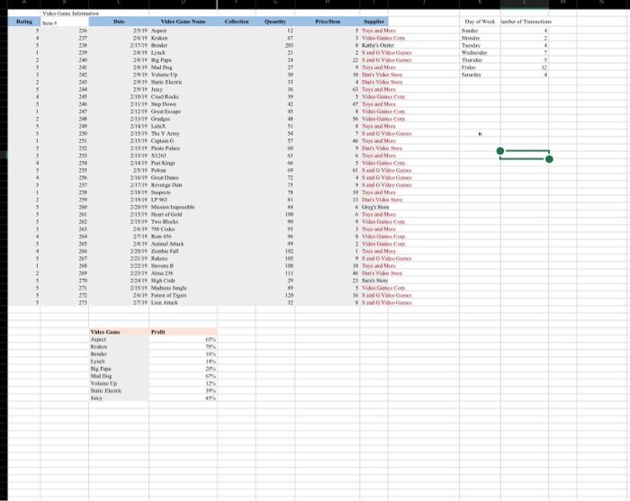
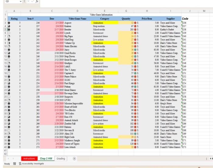
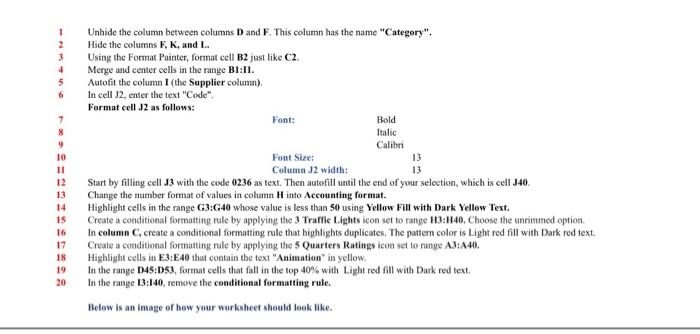
Unhide the column between columns D and F. This column has the name "Category". Hide the columns F,K, and L. Using the Format Painter, format cell B2 just like C2. Merge and center cells in the range B1:I1. Autofit the column 1 (the Supplier column). In cell J2, enter the text "Code". Format cell 32 as follows: Start by filling eell J3 with the code 0236 as text. Then autofill until the end of your selection, which is cell J40. Change the number format of values in column H into Accounting format. Highlight cells in the range G3:G40 whose value is less than 50 using Yellow Fill with Dark Yellow Text. Create a conditional formatting rule by applying the 3 Traffic Lights icon set to range H3:H40. Choose the unrimmed option. In column C, create a conditional formatting rule that highlights duplicates. The pattern color is Light red fill with Dark red text. Create a conditional formatting rule by applying the 5 Quarters Ratings icon set to nange A3:A40. Highlight cells in E3:E40 that contain the text "Animation" in yellow. In the range D45:D53, format cells that fall in the top 40% with Light red fill with Dark red text. In the range 13:140, remove the conditional formatting rule. Belew is an image of how your worksheet should look like. Unhide the column between columns D and F. This column has the name "Category". Hide the columns F,K, and L. Using the Format Painter, format cell B2 just like C2. Merge and center cells in the range B1:I1. Autofit the column 1 (the Supplier column). In cell J2, enter the text "Code". Format cell 32 as follows: Start by filling eell J3 with the code 0236 as text. Then autofill until the end of your selection, which is cell J40. Change the number format of values in column H into Accounting format. Highlight cells in the range G3:G40 whose value is less than 50 using Yellow Fill with Dark Yellow Text. Create a conditional formatting rule by applying the 3 Traffic Lights icon set to range H3:H40. Choose the unrimmed option. In column C, create a conditional formatting rule that highlights duplicates. The pattern color is Light red fill with Dark red text. Create a conditional formatting rule by applying the 5 Quarters Ratings icon set to nange A3:A40. Highlight cells in E3:E40 that contain the text "Animation" in yellow. In the range D45:D53, format cells that fall in the top 40% with Light red fill with Dark red text. In the range 13:140, remove the conditional formatting rule. Belew is an image of how your worksheet should look like