For reference:

RRP

HRP

factors.csv

dataset.csv

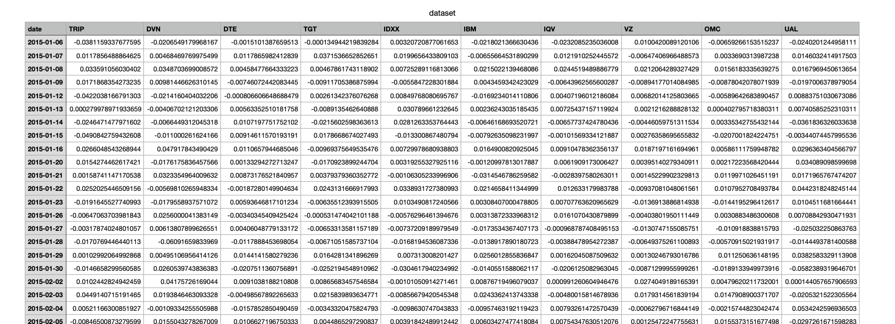
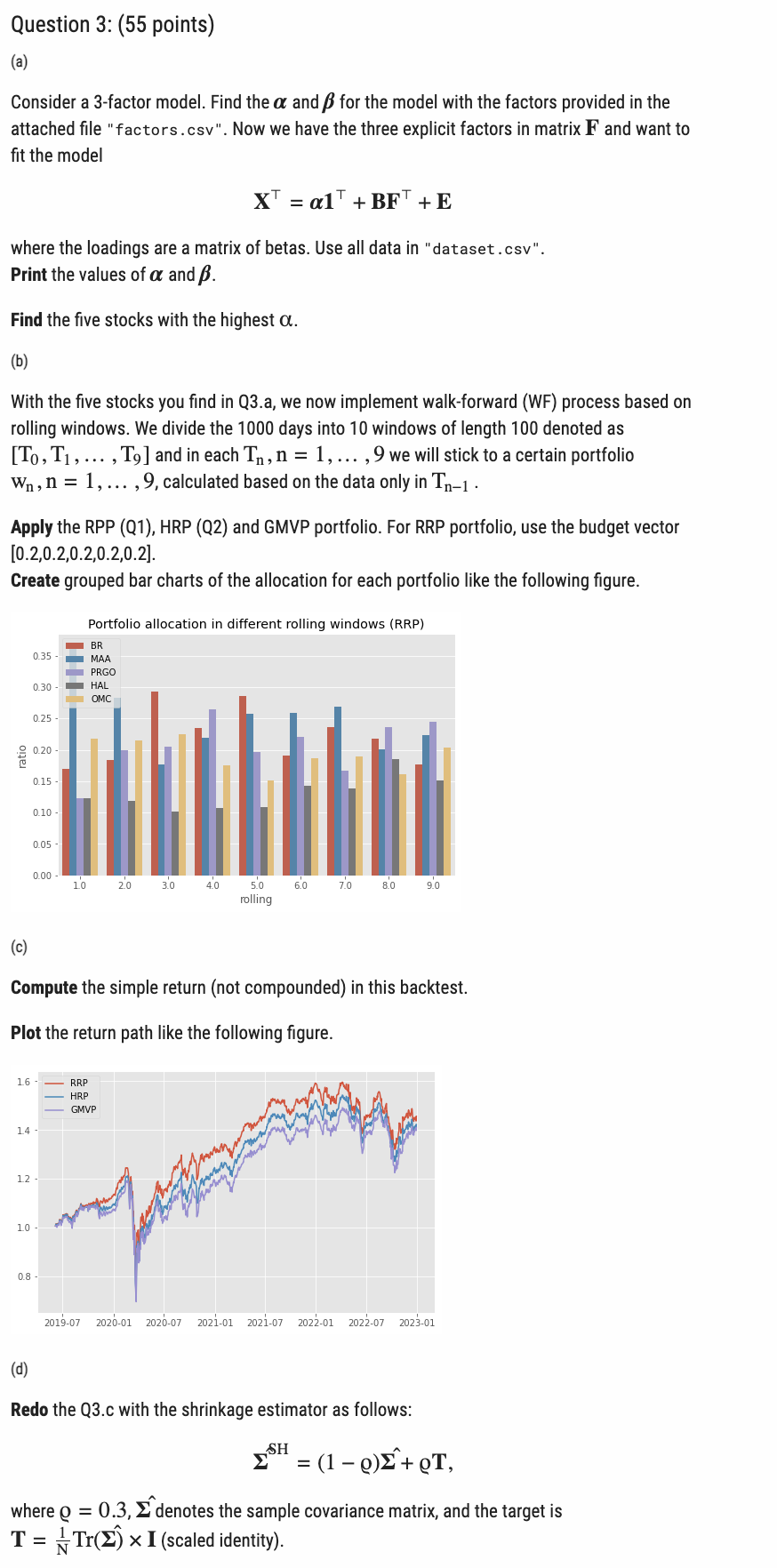
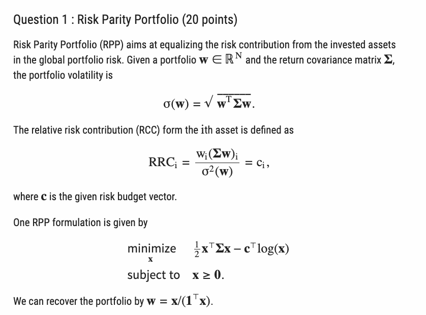
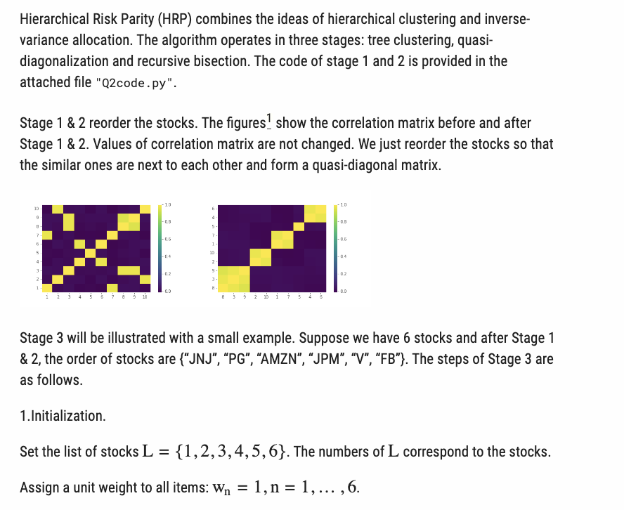
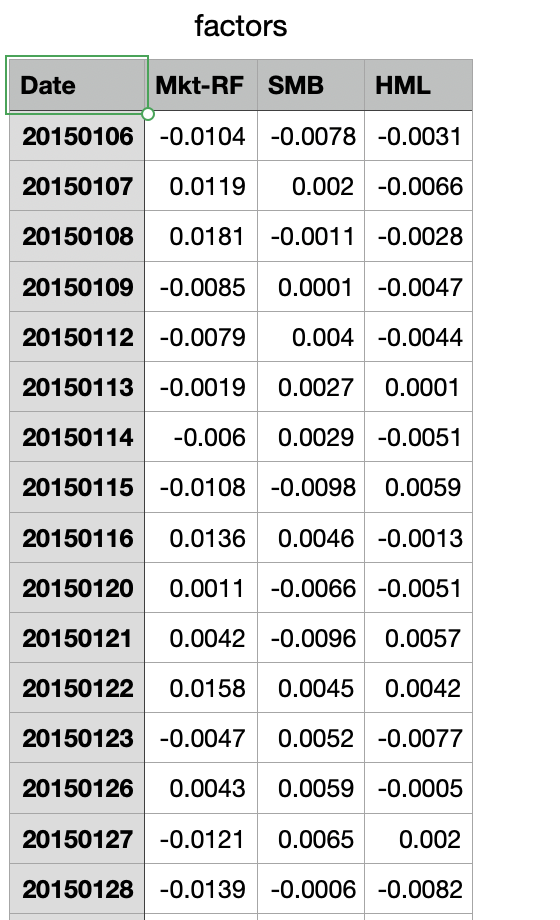
Consider a 3-factor model. Find the and for the model with the factors provided in the attached file "factors.csv". Now we have the three explicit factors in matrix F and want to fit the model X=1+BF+E where the loadings are a matrix of betas. Use all data in "dataset.csv". Print the values of and . Find the five stocks with the highest . (b) With the five stocks you find in Q3.a, we now implement walk-forward (WF) process based on rolling windows. We divide the 1000 days into 10 windows of length 100 denoted as [T0,T1,,T9] and in each Tn,n=1,,9 we will stick to a certain portfolio wn,n=1,,9, calculated based on the data only in Tn1. Apply the RPP (Q1), HRP (Q2) and GMVP portfolio. For RRP portfolio, use the budget vector [0.2,0.2,0.2,0.2,0.2] Create grouped bar charts of the allocation for each portfolio like the following figure. (c) Compute the simple return (not compounded) in this backtest. Plot the return path like the following figure. (d) Redo the Q3.c with the shrinkage estimator as follows: SH=(1)^+T where =0.3,^ denotes the sample covariance matrix, and the target is T=N1Tr(^)I(scaledidentity). Risk Parity Portfolio (RPP) aims at equalizing the risk contribution from the invested assets in the global portfolio risk. Given a portfolio wRN and the return covariance matrix , the portfolio volatility is (w)=wTw The relative risk contribution (RCC) form the ith asset is defined as RRCi=2(w)wi(w)i=ci where c is the given risk budget vector. One RPP formulation is given by xminimizesubjectto21xxclog(x)x0. We can recover the portfolio by w=x/(1x). Hierarchical Risk Parity (HRP) combines the ideas of hierarchical clustering and inversevariance allocation. The algorithm operates in three stages: tree clustering, quasidiagonalization and recursive bisection. The code of stage 1 and 2 is provided in the attached file "Q2code.py". Stage 1&2 reorder the stocks. The figures_ 1 show the correlation matrix before and after Stage 1&2. Values of correlation matrix are not changed. We just reorder the stocks so that the similar ones are next to each other and form a quasi-diagonal matrix. Stage 3 will be illustrated with a small example. Suppose we have 6 stocks and after Stage 1 &2, the order of stocks are { "JNJ", "PG", "AMZN", "JPM", "V", "FB"\}. The steps of Stage 3 are as follows. 1.Initialization. Set the list of stocks L={1,2,3,4,5,6}. The numbers of L correspond to the stocks. Assign a unit weight to all items: wn=1,n=1,,6. factors \begin{tabular}{|l|r|r|r|} \hline Date & Mkt-RF & \multicolumn{1}{|l|}{ SMB } & \multicolumn{1}{l|}{ HML } \\ \hline 20150106 & -0.0104 & -0.0078 & -0.0031 \\ \hline 20150107 & 0.0119 & 0.002 & -0.0066 \\ \hline 20150108 & 0.0181 & -0.0011 & -0.0028 \\ \hline 20150109 & -0.0085 & 0.0001 & -0.0047 \\ \hline 20150112 & -0.0079 & 0.004 & -0.0044 \\ \hline 20150113 & -0.0019 & 0.0027 & 0.0001 \\ \hline 20150114 & -0.006 & 0.0029 & -0.0051 \\ \hline 20150115 & -0.0108 & -0.0098 & 0.0059 \\ \hline 20150116 & 0.0136 & 0.0046 & -0.0013 \\ \hline 20150120 & 0.0011 & -0.0066 & -0.0051 \\ \hline 20150121 & 0.0042 & -0.0096 & 0.0057 \\ \hline 20150122 & 0.0158 & 0.0045 & 0.0042 \\ \hline 20150123 & -0.0047 & 0.0052 & -0.0077 \\ \hline 20150126 & 0.0043 & 0.0059 & -0.0005 \\ \hline 20150127 & -0.0121 & 0.0065 & 0.002 \\ \hline 20150128 & -0.0139 & -0.0006 & -0.0082 \\ \hline \end{tabular} Consider a 3-factor model. Find the and for the model with the factors provided in the attached file "factors.csv". Now we have the three explicit factors in matrix F and want to fit the model X=1+BF+E where the loadings are a matrix of betas. Use all data in "dataset.csv". Print the values of and . Find the five stocks with the highest . (b) With the five stocks you find in Q3.a, we now implement walk-forward (WF) process based on rolling windows. We divide the 1000 days into 10 windows of length 100 denoted as [T0,T1,,T9] and in each Tn,n=1,,9 we will stick to a certain portfolio wn,n=1,,9, calculated based on the data only in Tn1. Apply the RPP (Q1), HRP (Q2) and GMVP portfolio. For RRP portfolio, use the budget vector [0.2,0.2,0.2,0.2,0.2] Create grouped bar charts of the allocation for each portfolio like the following figure. (c) Compute the simple return (not compounded) in this backtest. Plot the return path like the following figure. (d) Redo the Q3.c with the shrinkage estimator as follows: SH=(1)^+T where =0.3,^ denotes the sample covariance matrix, and the target is T=N1Tr(^)I(scaledidentity). Risk Parity Portfolio (RPP) aims at equalizing the risk contribution from the invested assets in the global portfolio risk. Given a portfolio wRN and the return covariance matrix , the portfolio volatility is (w)=wTw The relative risk contribution (RCC) form the ith asset is defined as RRCi=2(w)wi(w)i=ci where c is the given risk budget vector. One RPP formulation is given by xminimizesubjectto21xxclog(x)x0. We can recover the portfolio by w=x/(1x). Hierarchical Risk Parity (HRP) combines the ideas of hierarchical clustering and inversevariance allocation. The algorithm operates in three stages: tree clustering, quasidiagonalization and recursive bisection. The code of stage 1 and 2 is provided in the attached file "Q2code.py". Stage 1&2 reorder the stocks. The figures_ 1 show the correlation matrix before and after Stage 1&2. Values of correlation matrix are not changed. We just reorder the stocks so that the similar ones are next to each other and form a quasi-diagonal matrix. Stage 3 will be illustrated with a small example. Suppose we have 6 stocks and after Stage 1 &2, the order of stocks are { "JNJ", "PG", "AMZN", "JPM", "V", "FB"\}. The steps of Stage 3 are as follows. 1.Initialization. Set the list of stocks L={1,2,3,4,5,6}. The numbers of L correspond to the stocks. Assign a unit weight to all items: wn=1,n=1,,6. factors \begin{tabular}{|l|r|r|r|} \hline Date & Mkt-RF & \multicolumn{1}{|l|}{ SMB } & \multicolumn{1}{l|}{ HML } \\ \hline 20150106 & -0.0104 & -0.0078 & -0.0031 \\ \hline 20150107 & 0.0119 & 0.002 & -0.0066 \\ \hline 20150108 & 0.0181 & -0.0011 & -0.0028 \\ \hline 20150109 & -0.0085 & 0.0001 & -0.0047 \\ \hline 20150112 & -0.0079 & 0.004 & -0.0044 \\ \hline 20150113 & -0.0019 & 0.0027 & 0.0001 \\ \hline 20150114 & -0.006 & 0.0029 & -0.0051 \\ \hline 20150115 & -0.0108 & -0.0098 & 0.0059 \\ \hline 20150116 & 0.0136 & 0.0046 & -0.0013 \\ \hline 20150120 & 0.0011 & -0.0066 & -0.0051 \\ \hline 20150121 & 0.0042 & -0.0096 & 0.0057 \\ \hline 20150122 & 0.0158 & 0.0045 & 0.0042 \\ \hline 20150123 & -0.0047 & 0.0052 & -0.0077 \\ \hline 20150126 & 0.0043 & 0.0059 & -0.0005 \\ \hline 20150127 & -0.0121 & 0.0065 & 0.002 \\ \hline 20150128 & -0.0139 & -0.0006 & -0.0082 \\ \hline \end{tabular}