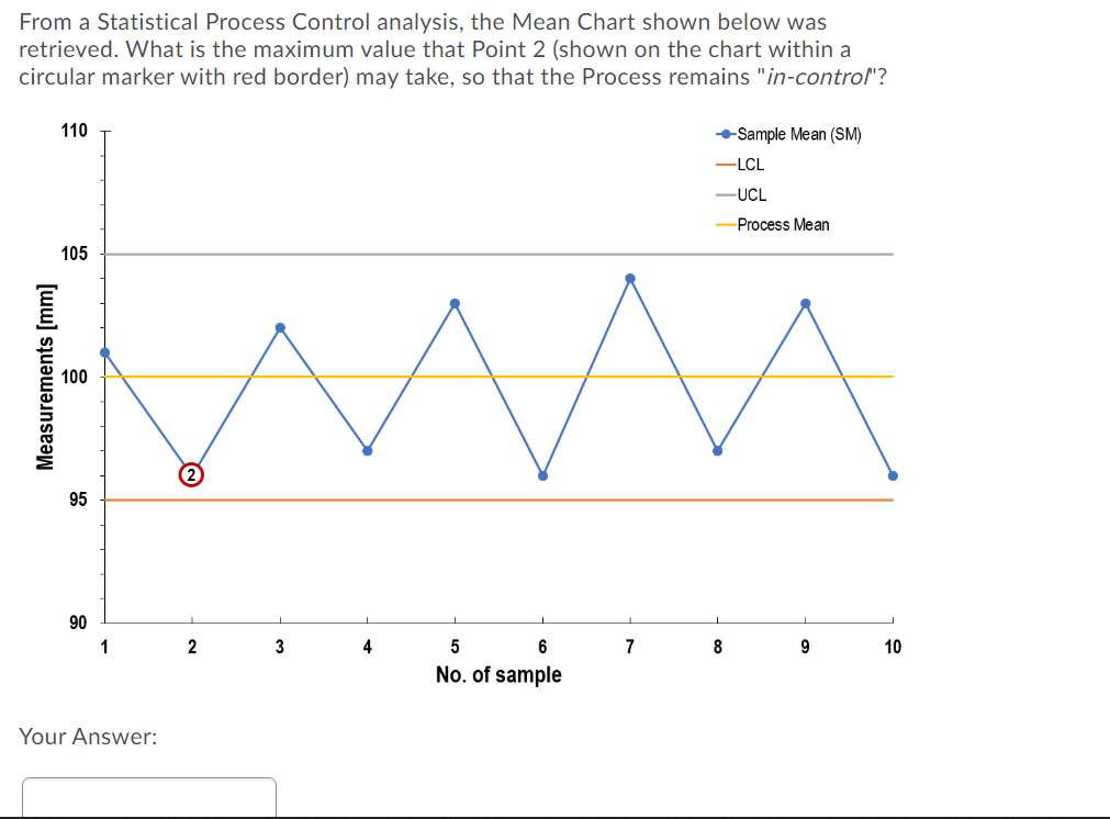
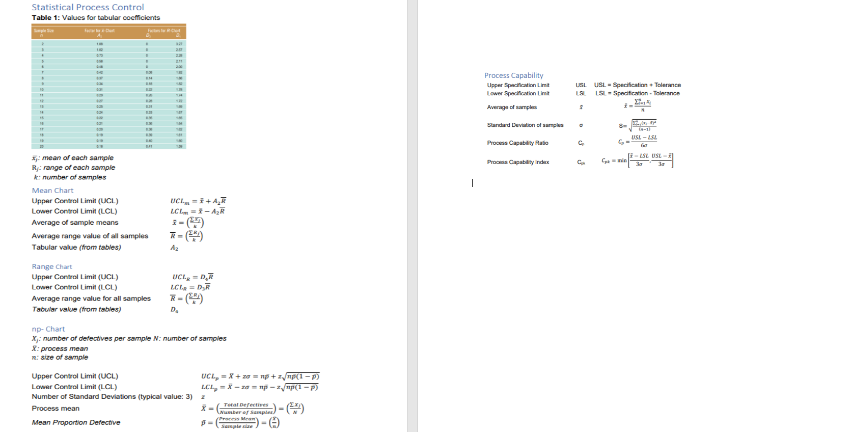
Question: From a Statistical Process Control analysis, the Mean Chart shown below was retrieved. What is the maximum value that Point 2 (shown on the chart

From a Statistical Process Control analysis, theFrom a Statistical Process Control analysis, theFrom a Statistical Process Control analysis, the

From a Statistical Process Control analysis, the Mean Chart shown below was retrieved. What is the maximum value that Point 2 (shown on the chart within a circular marker with red border) may take, so that the Process remains "in-control"? 110 -Sample Mean (SM) -LCL -UCL Process Mean 105 Measurements [mm] 100 AMA @ 95 90 1 2 3 4 7 8 9 10 5 6 No. of sample Your Answer: Tables & List of Equations 7: high (overall reduced performance) 8: very high (product inoperable, loss of primary function) 9: hazardous (damage to people) 10: hazardous (no warning!) 8: high 1:8 9: very high 1:3 10: very high 1:2 8: Remote 9: Very Remote 10: Absolute uncertainty Kano Model System Reliability OPTIONS L Like it E Expect it N Neutral T Tolerate it D Dislike it Components in Parallel Kano DYSFUNCTIONAL model LENT D LQAAA P ERUIUM NRIT 1 M TR 1 1 1 M DRRRRQ FEATURE CLASSIFICATION M Must-Be P Performance A Attractive Indifferent Q Questionable (invalid) R Reversal (invalid) Backup 0.90 R Components in Series 0.90 0.90 Original - 0.95 - R 0.95 + (1 -0.95)(0.90) = 0.995 + (= 0.90 x 0.90 = 0.81 R = (R.) *(R) *... (R) R: reliability of n-th component. R=R, + (1 - R,)*(R) Analytic Hierarchy Process (AHP) Intensity of Definition Explanation on an absolute scale importance 1 Equal importance Two activities contribute equally to the objective 3 Moderate importance of one another Experience and judgment strongly favour one activity over another Experience and judgement strongly favour one 5 Essential or Strong importance activity over another An activity is strongly favoured and its dominance 7 7 Very strong importance demonstrated in practice 9 Extreme importance The evidence favouring one activity over another is of the highest possible order or affirmation Intermediate values between the two 2,4,6,8 adjacent judgments When compromise is needed Reciprocals If activity i has one of the above numbers assigned to it when compared with activity j, then Rationals Ratios arising from the scale If consistency were to be forced by obtaining n numerical values to span the matrix Mean Time Between Failures (MTBF): Length of time a product / service is in operation before it )/ fails Mean Time To Repair (MTTR): Length of time required to set a product / service back in operation System Availability (SA): % of time a product or service is in operation MTBF SA= MTBF + MTTR Cost of Quality TQC = CC + NCC + CC = PC+ACTFL = IFC + EFC NCC = TFL TQC: Total Quality Cost CC.Conformance Cost NCC:Non-Conformance Cost PC: Prevention Cost AC: Appraisal Cost TFC: Total Failure Cost IFC: Internal Failure Cost EFC: External Failure Cost Failure Mode and Effect Analysis RPN = Sx XD RPN: Risk Priority Number S: Severity o: Occurrence D: Detection Rating for Severity Rating for Occurrence 1: no effect 1: remote 1s 1,500,000 2: very minor (discerning customers) 2: low 1: 150.000 3: minor (average customers) 3 3: low 1:15,000 4: very low (most customers) 4: moderate 1:2.000 5: low (product functions, minor features 5: moderate 1: 400 have reduced performance) 6: moderate 1: 80 6: moderate (all minor features fail) 7: high 1:20 Labor Index = Quality Cost Direct Labor Hours Rating for Detection 1: Almost certain 2: Very high 3: High 4: Moderately High 5: Moderate 6: Low 7: Very Low Cost Index = Quality Cost Manufacturing Cost Quality Cost Sales Index = Quality Cost Production Index = units of Final Product Sales Statistical Process Control Table 1: Values for tabular coefficients Sample Se Factor for X-Chart Factors for R-Chart A D D 2 2.57 . . 0.73 4 5 B T 8 04 2.11 200 182 0.00 0.14 0.18 182 Process Capability Upper Specification Limit Lower Specification Limit 10 11 0:31 USL USL = Specification + Tolerance LSL LSL = Specification - Tolerance 174 1.72 O2T x 12 13 0.31 Average of samples * i=114 n 157 0.24 0:22 0:21 Standard Deviation of samples g 14 15 16 17 18 19 20 0.35 03 08 0 0.0 0.41 1 161 019 0.16 Process Capability Ratio C 2.(x-2) x S (n-1) USL - LSL C Cp 60 3 - LSL USL - ] Cpk = min 30 Process Capability Index Cpk | xmean of each sample Rj: range of each sample k: number of samples Mean Chart Upper Control Limit (UCL) Lower Control Limit (LCL) Average of sample means Average range value of all samples Tabular value (from tables) ) UCLm = * +AR LCL m = * -AR i= R= A2 Range Chart Upper Control Limit (UCL) Lower Control Limit (LCL) Average range value for all samples Tabular value (from tables) UCLR = D.R LCLR = DR R = D np-Chart X: number of defectives per sample : number of samples X: process mean n: size of sample Upper Control Limit (UCL) Lower Control Limit (LCL) Number of Standard Deviations (typical value: 3) Process mean Mean Proportion Defective UCL = x + zo = np + z.p(1-7) LCL = X - zo = np - zp(1-D z X= Total Defectives Number of Samples =6) Process Mean P= = Sample size)

Step by Step Solution

There are 3 Steps involved in it

1 Expert Approved Answer
Step: 1 Unlock blur-text-image
Question Has Been Solved by an Expert!

Get step-by-step solutions from verified subject matter experts

Step: 2 Unlock
Step: 3 Unlock

Students Have Also Explored These Related General Management Questions!