.....help me understand this

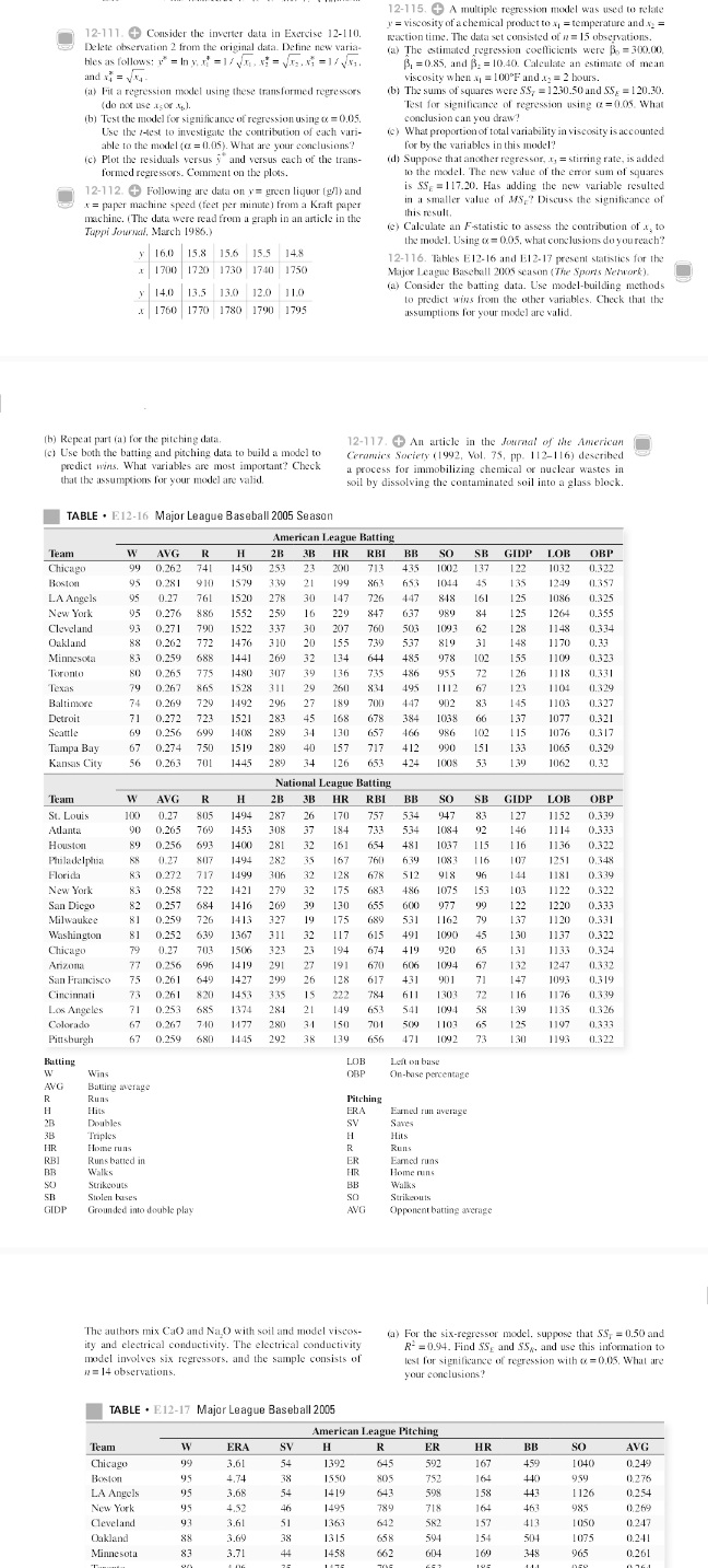
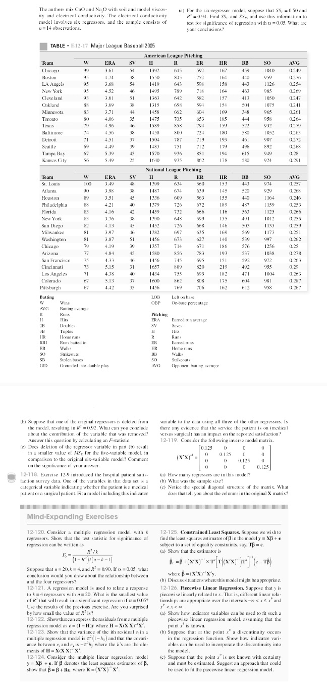
12-115. + A multiple regression model was used to relate y' = viscosity of a chemical product toy = temperature and = 12-111. + Consider the inverter data in Exercise 12-110. reaction time. The data set consisted of n = 15 observations. Delete observation 2 from the original data. Define new varia- (@) The estimated regression coefficients were Bo = 300.00. bles as follows: v' = In y. x) = 1/ vn , x = V.12 . Ni =1/ VN. 3, =0.85, and 5, = 10.40. Calculate an estimate of mean and 1 = VS. viscosity when * = 100 F and .to = 2 hours. (a) Fit a regression model using these transformed regressors (b) The sums of squares were SS, = 1230.50 and $5, = 120.30. (do not use agor &;). Test for significance of regression using a =0.05. What (bj Test the model for significance of regression using o = 0.05. conclusion can you draw? Use the /test to investigate the contribution of each vari- (c) What proportion of total variability in viscosity is accounted able to the model (c = 0.05). What are your conclusions? for by the variables in this model? (c) Plot the residuals versus ;" and versus each of the trans- (d) Suppose that another regressor, I, = stirring rate, is added formed regressors. Comment on the plots. to the model. The new value of the error sum of squares 12-112. + Following are data on y'= green liquor (g/1) and Is $S= = 117.20. Has adding the new variable resulted * = paper machine speed (feet per minute) from a Kraft paper n a smaller value of MS, ? Discuss the significance of this result. machine. (The data were read from a graph in an article in the fe) Calculate an Fstatistic to assess the contribution of a, to Toppi Journal, March 1986.) the model. Using o = 0.05, what conclusions do you reach? 16.0 15.8 15.6 15.5 148 12-116. Tables E12-16 and B1 2-17 present statistics for the 1 1700 1720 1730 1740 1750 Major League Baseball 2005 season (The Sports Network). (a) Consider the batting data. Use model-building methods y 140 13.5 13.0 12.0 11.0 to predict wins from the other variables. Check that the .4 1760 1770 1780 1790 1795 assumptions for your model are valid. (b) Repeat part (a) for the pitching data, 12-117. + An article in the Journal of the American (c) Use both the batting and pitching data to build a model to Ceramics Society (1992, Vol. 75, pp. 112-116) described predict wins. What variables are most important? Check a process for immobilizing chemical or nuclear wastes in that the assumptions for your model are valid. soil by dissolving the contaminated soil into a glass block. TABLE . E12-16 Major League Baseball 2005 Season American League Batting Team W AVG R H 2B 3B HR RBI BB SO SB GIDP LOB OBP Chicago 99 0.262 741 1450 253 23 200 713 435 1002 137 122 1032 0.327 Boston 95 0.281 910 3.39 21 199 863 653 1044 45 135 1249 0.357 LA Angels 0.27 761 1520 278 30 147 726 447 818 161 125 1086 0.325 New York 0.276 $86 155 259 16 229 847 637 080 84 125 1264 0.355 Cleveland 0.271 790 1522 337 30 207 760 503 1093 62 128 1148 0.334 Oakland 0.262 772 1476 310 20 155 739 537 819 31 148 1170 0.33 Minnesota 83 0.259 688 144 269 32 134 644 485 978 102 155 1109 0.323 Toronto 10 0.265 775 1480 307 39 136 735 486 955 72 126 1118 0,331 Texas 0.267 865 1528 311 29 260 834 195 1112 63 123 1 104 0.329 Baltimore 74 0.269 729 1492 206 27 189 700 147 on2 83 145 1103 0.327 Detroit 71 0).272 723 1521 283 45 168 678 384 1038 66 137 1077 0.321 Seattle 0.256 699 1408 289 34 130 657 986 102 1 15 1076 0.317 Tampa Bay 0.274 750 1519 289 40 157 717 12 090 151 133 1065 0.325 Kansas City 56 0.263 701 1445 289 34 126 653 424 1008 53 139 1062 0,32 National League Batting Team W AVG R H 213 3B HR RBI BB SB GIDP LOB OBP St. Louis 100 0.27 805 1494 287 26 170 757 534 947 83 127 1152 0.3.39 Atlanta 90 0.265 769 145 308 37 184 733 534 1084 92 146 11 14 0.333 Houston 59 0.256 693 1400 281 32 161 654 481 1037 115 1 16 1136 0.327 Philadelphia 0.27 807 149 282 35 760 1083 1 16 107 1251 Florida 83 0.272 717 1494 306 32 128 638 $17 918 96 144 1181 0.379 New York 33 0.258 722 1421 279 32 175 683 486 1075 153 103 1122 0.327 San Diego 32 0.257 684 1416 269 39 130 655 600 977 99 122 1220 1.333 Milwaukee 31 0.259 726 1413 327 19 175 689 531 1 162 79 137 1120 0.331 Washington 81 0.252 639 1367 311 32 117 615 491 1090 45 130 1137 0.327 Chicago 0.27 703 1506 323 23 194 674 419 920 65 131 1133 0.324 Arizona 77 0,256 696 1419 291 27 191 630 606 1094 67 132 1247 0.337 San Francisco 75 0.261 649 1427 299 26 128 617 431 901 71 147 1093 0.319 Cincinnati 73 0,261 8201 1453 335 IS 222 784 611 130 72 1 16 1176 11,339 Los Angeles 0.253 685 1374 284 21 149 653 541 1094 58 139 1135 11.326 Colorado 0,267 740 1477 280 31 150 70 500 1103 65 125 1197 0.373 Pittsburgh 0.259 680 1445 292 130 656 171 1092 73 130 1193 0.322 Hatting LOB Left on base Wins OBP On-base percentage AVG Baking average Runs Pitching Hits ERA Earned run average 28 Doubles SV Saves Triple H Hits HR Home runs Run BBI Runs batted in Earned runs BR Walks FIR Home runs SO Strikeouts BB Walk 5B Stolen bases 50 Strikeouts GIOP Grounded into double play AVG Opponent batting average The authors mix CaO and Na,O with soil and model viscos- (a) For the six-regressor model. suppose that SS, = 0.50 and ty and electrical conductivity. The electrical conductivity R- =0.94. Find $5, and $5,, and use this information to model involves six repressors, and the sample consists of test for significance of regression with o = 0.05. What are 1 = 14 observations. your conclusions? TABLE . E12-17 Major League Baseball 2005 American League Pitching Team W ERA SV H R ER HR BB SO AVG Chicago 3.61 54 1392 645 592 167 459 1040 0.249 Boston 15 4,74 38 1550 805 752 164 4 40) 454 0.276 LA Angels 15 3.68 54 141 643 598 158 443 126 0.254 New York 4,52 46 149 789 718 164 463 985 0,269 Cleveland 43 3.61 51 1363 642 582 157 415 1050 0.247 Oakland 88 3.69 1315 658 594 154 504 075 0.241 Minnesota 83 3.71 1458 662 604 160 348 965 0.261The authors mix CaO and Na, O with soil and model viscos- () For the six-regressor model, suppose that SS, = 0.50 and ity and electrical conductivity. The electrical conductivity R- =0.94. Find $5, and $5,, and use this information to model involves six regressors, and the sample consists of test for significance of regression with o = 0.05. What are n = 14 observations. your conclusions? TABLE . E12-17 Major League Baseball 2006 American League Pitching Tean W ERA SV H R ER HR BB SO AVG Chicago 99 3.61 54 1392 645 592 167 459 1040 0.249 Boston 95 4,74 38 1550 805 752 164 440 959 0.276 LA Angels 95 3.68 54 1419 643 598 158 443 1 126 0.254 New York 95 4.52 46 1495 789 718 164 463 985 0.269 Cleveland 93 3.6 51 1363 642 582 157 413 1050 0.247 Oakland 88 3.64 38 1315 658 594 154 1075 0.241 Minnesota 83 3.71 44 1458 662 GD4 169 348 965 0.261 Toronto 4.06 35 1475 705 653 185 414 958 0.264 Texas 79 4.96 46 1589 858 794 159 522 932 0.279 Baltimore 74 4.56 38 1458 800 724 180 580 1052 0.263 Detroit 71 4.51 37 1504 787 719 193 461 907 0.272 Seattle 69 4,49 39 1483 751 712 179 495 892 0.268 Tampa Bay 67 5.39 43 1570 936 851 194 949 0.28 Kansas City 56 5.49 25 1640 935 862 178 580 924 0.291 National League Pitching Team W ERA SV H R ER HR BB SO AVG St. Louis 100 3.45 48 1 399 634 560 153 443 974 0.257 Atlanta 90 3.98 38 1487 674 639 145 520 929 0. 268 Houston 3.51 45 1336 509 563 155 440 1 164 0.246 Philadelphia 58 4,21 40 1370 726 672 189 487 1 159 0.253 Florida 4.16 42 1450 732 666 116 563 1 125 0.266 New York 83 3.36 38 1 390 648 599 135 491 1012 0.255 San Diego 82 4.13 45 1452 726 668 146 503 1133 0.259 Milwaukee 8I 3.97 46 1 382 697 635 169 564 1175 0.251 Washington 81 3.87 51 1456 673 627 140 539 0.262 Chicago 4.19 39 1357 714 671 186 576 1256 0.25 Arizona 77 4.84 45 1580 856 783 193 537 1038 0.278 San Francisco 75 4.33 46 1456 745 695 151 592 972 0.263 Cincinnati 73 5.14 31 1657 889 820 219 492 955 0,29 Los Angeles 71 4.38 40 1434 755 695 182 471 1004 0.263 Colorado 657 5.13 37 1600 862 808 175 604 981 0.287 Pillsburgh 63 142 35 1456 760 706 162 612 958 0.267 Batting LOB Left on base W Wins OBF On-base percentage AVG Bating average R Run Pitching Hits ERA Earned run average Doubles SV Saves Triples Hits HR Home runs R Runs RBI Runs batted in ER Earned runs BR Walks HE Home runs SO Strikeouts BE Walks Stolen bases 50 Strikeouts GID Grounded into double play AVC Opponent batting average (b) Suppose that one of the original regressors is deleted from variable to the data using all three of the other regressors. Is the model, resulting in R- =0.92. What can you conclude there any evidence that the service the patient is on (medical about the contribution of the variable that was removed? versus surgical) has an impact on the reported satisfaction? Answer this question by calculating an F-statistic. 12-119. Consider the following inverse model matrix. (c) Does deletion of the regressor variable in pant (b) result [0.125 0) in a smaller value of MS, for the five-variable model. in comparison to the original six-variable model? Comment (XX) = 0.125 0 0.125 on the significance of your answer. 0.125 12-118. Exercise 12-9 introduced the hospital patient satis- (a) How many regressors are in this model? action survey data. One of the variables in that data set is a (b) What was the sample size? categorical variable indicating whether the patient is a medical (c) Notice the special diagonal structure of the matrix, What patient or a surgical patient. Fit a model including this indicator does that tell you about the columns in the original X matrix? Mind-Expanding Exercises 12-120. Consider a multiple regression model with & 12-125. Constrained Least Squares. Suppose we wish to regressors. Show that the test statistic for significance of find the least squares estimator of B in the model y = XP + e regression can be written as subject to a set of equality constraints, say, TB = c. (a) Show that the estimator is Fo (1 -R]] /[n- K-1) B. =B+(XX)"XT T[(xx)'T|(c-19) Suppose that a = 20.