Here's the starter matlab code

% quadratic fitting

% 1) generate an exact cubic: close all; clear all; clc a = 5; b = 3; c = 5; d = -1; xs = -1:.01:1; % mesh of x values from -3 to 2 n = length(xs); % number of points xs = reshape(xs, n, 1); %I want a column vector

yTrue = a*xs.^3 + b*xs.^2 + c*xs + d; % y values (same size as xs) yNoisy = yTrue + 4*randn(n, 1); % now, we add some random noise to wiggle the curve

% now we fit a 3rd degree polynomial to noisy data. A = [xs.^15 xs.^14 xs.^13 xs.^12 ... xs.^11 xs.^10 xs.^9 ... xs.^8 xs.^7 xs.^6 xs.^5 xs.^4 xs.^3 xs.^2 xs ones(n,1)]; b = yNoisy; sol = (A'*A)\(A'*b); [m,n] = size(A);

D = diag(n:-1:1).^2; solReg = (A'*A + D)\(A'*b); % solution from Hw5 lambda = 1; tol = 1e-2; maxIter = 50000;

% write code to compute solL1 here

% iterate the loop until norm(solL1 - solL1old)*L

% your solution should be called solL1 % then code below will plot everything.

predictedYs = A*sol; predictedYsReg = A*solReg; predictedYsL1 = A*solL1;

plot(xs, yTrue, 'k', 'LineWidth',2) % plots true curve hold on % waits for more %plot(xs, yNoisy, 'ro') plot(xs, predictedYs, '--r', 'LineWidth', 2) plot(xs, predictedYsReg, '-.g', 'LineWidth', 2) plot(xs, predictedYsL1, '-.b', 'LineWidth', 2)

legend('true undelrying curve', 'noisy realizations', 'fitted polynomial', 'l1-fit', 'Location','northwest')

% makes an eps figure print('PolyFit','-depsc'

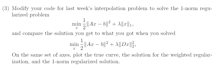
(3) Modify your code for last week's interpolation problem to solve the 1-norm regu larized problem mln. Aar bll2 Allarll1, and compare the solution you get to what you got when you solved min. On the same set of axes, plot the true curve, the solution for the weighted regular- ization, and the 1-norm regularized solution