Please help modifying this given code. This is a Matlab question. Clear code with explanation.

--------------------------------------- close all; clear; clc;

set(groot,'defaultAxesTickLabelInterpreter','latex');

set(groot,'defaulttextinterpreter','latex'); set(groot,'defaultLegendInterpreter','latex'); %% The following data are from the U.S. Standard Atmosphere 1976 model % altitude (km) above the Earth's sea level h = [0:1:10, 15:5:30, 40:10:80]'; % average temperature (degree Celcicus) above the Earth's sea level T = [15 8.5 2 -4.49 -10.98 -17.47 -23.96 -30.45 -36.94 -43.42 -49.90 ... -56.50 -56.50 -51.60 -46.64 -22.80 -2.5 -26.13 -53.57 -74.51]'; % plot the datapoints figure(1) scatter(T,h,140,'bo','MarkerEdgeColor','k',... 'MarkerFaceColor','k','MarkerFaceAlpha',0.4) hold on set(gca,'FontSize',30) xlabel('temperature (degree Celcius)','FontSize',25); ylabel('altitude (km)','FontSize',25); %% compute and plot the spline interpolants h_query = linspace(min(h),max(h),200); line_color = {'r','g','b'}; line_style = {'-','-.','--'}; % your code here to compute and plot the linear, quadratic and cubic % splines, together with the datapoints in the same figure window % you can write as many lines of code as you want in this segment legend('datapoints','linear spline','quadratic spline','cubic spline')

------------------------------------------------------------------------------

This above is the given HW6p1.m file

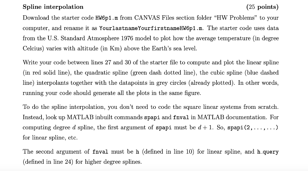
Spline interpolation (25 points) Download the starter code HW6p1.m from CANVAS Files section folder HW Problems to your computer, and rename it as Yourlastname Yourfirstname HW6p1.m. The starter code uses data from the U.S. Standard Atmosphere 1976 model to plot how the average temperature (in degree Celcius) varies with altitude (in Km) above the Earth's sea level. Write your code between lines 27 and 30 of the starter file to compute and plot the linear spline (in red solid line), the quadratic spline (green dash dotted line), the cubic spline (blue dashed line) interpolants together with the datapoints in grey circles (already plotted). In other words, running your code should generate all the plots in the same figure. To do the spline interpolation, you don't need to code the square linear systems from scratch. Instead, look up MATLAB inbuilt commands spapi and fnval in MATLAB documentation. For computing degree d spline, the first argument of spapi must be d+1. So, spapi(2,...,...) for linear spline, etc. The second argument of fnval must be h (defined in line 10) for linear spline, and h_query (defined in line 24) for higher degree splines. Spline interpolation (25 points) Download the starter code HW6p1.m from CANVAS Files section folder HW Problems to your computer, and rename it as Yourlastname Yourfirstname HW6p1.m. The starter code uses data from the U.S. Standard Atmosphere 1976 model to plot how the average temperature (in degree Celcius) varies with altitude (in Km) above the Earth's sea level. Write your code between lines 27 and 30 of the starter file to compute and plot the linear spline (in red solid line), the quadratic spline (green dash dotted line), the cubic spline (blue dashed line) interpolants together with the datapoints in grey circles (already plotted). In other words, running your code should generate all the plots in the same figure. To do the spline interpolation, you don't need to code the square linear systems from scratch. Instead, look up MATLAB inbuilt commands spapi and fnval in MATLAB documentation. For computing degree d spline, the first argument of spapi must be d+1. So, spapi(2,...,...) for linear spline, etc. The second argument of fnval must be h (defined in line 10) for linear spline, and h_query (defined in line 24) for higher degree splines