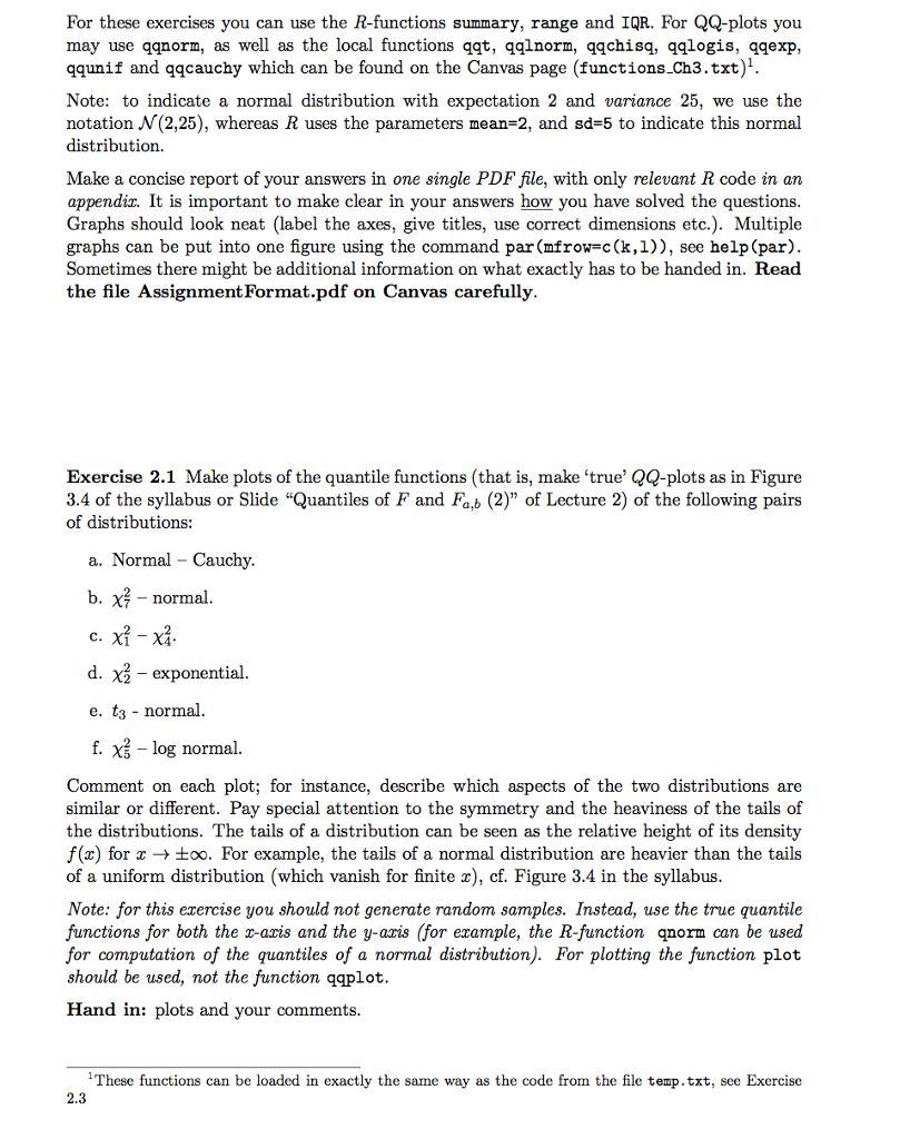
Question: Hi, can you answer the following question with code for R studio. Also can you use the plot commnad when making the graphs. For these
Hi, can you answer the following question with code for R studio. Also can you use the "plot" commnad when making the graphs. 
For these exercises you can use the R-functions summary, range and IQR. For QQ-plots you may use qqnorm, as well as the local functions qqt, qqlnorm, qqchisq, qqlogis, qqexp qqunif and qqcauchy which can be found on the Canvas page (functions_Ch3.txt)1 Note: to indicate a normal distribution with expectation 2 and variance 25, we use the notation (2,25), whereas R uses the parameters mean-2, and sd-5 to indicate this normal distribution Make a concise report of your answers in one single PDF file, with only relevant R code in a:n appendiz. It is important to make clear in your answers how you have solved the questions Graphs should look neat (label the axes, give titles, use correct dimensions etc.). Multiple graphs can be put into one figure using the command par(mfrow-c(k,1)), see help (par) Sometimes there might be additional information on what exactly has to be handed in. Read the file Assignment Format.pdf on Canvas carefully Exercise 2.1 Make plots of the quantile functions (that is, make 'true' QQ-plots as in Figure 3.4 of the syllabus or Slide "Quantiles of F and Fab (2)" of Lecture 2) of the following pairs of distributions: a. Normal- Cauchy bx?-normal X5-exponential. e. t3-normal f. x% -log normal. Comment on each plot; for instance, describe which aspects of the two distributions are similar or different. Pay special attention to the symmetry and the heaviness of the tails of the distributions. The tails of a distribution can be seen as the relative height of its density f(x) for x oo. For example, the tails of a normal distribution are heavier than the tails of a uniform distribution (which vanish for finite x), cf. Figure 3.4 in the syllabus Note: for this exercise you should not generate random samples. Instead, use the true quantile functions for both the r-axis and the y-aris (for example, the R-function qnorm can be used for computation of the quantiles of a normal distribution). For plotting the function plot should be used, not the function qqplot Hand in: plots and your comments These functions can be loaded in exactly the same way as the code from the file temp.txt, see Exercise 2.3 For these exercises you can use the R-functions summary, range and IQR. For QQ-plots you may use qqnorm, as well as the local functions qqt, qqlnorm, qqchisq, qqlogis, qqexp qqunif and qqcauchy which can be found on the Canvas page (functions_Ch3.txt)1 Note: to indicate a normal distribution with expectation 2 and variance 25, we use the notation (2,25), whereas R uses the parameters mean-2, and sd-5 to indicate this normal distribution Make a concise report of your answers in one single PDF file, with only relevant R code in a:n appendiz. It is important to make clear in your answers how you have solved the questions Graphs should look neat (label the axes, give titles, use correct dimensions etc.). Multiple graphs can be put into one figure using the command par(mfrow-c(k,1)), see help (par) Sometimes there might be additional information on what exactly has to be handed in. Read the file Assignment Format.pdf on Canvas carefully Exercise 2.1 Make plots of the quantile functions (that is, make 'true' QQ-plots as in Figure 3.4 of the syllabus or Slide "Quantiles of F and Fab (2)" of Lecture 2) of the following pairs of distributions: a. Normal- Cauchy bx?-normal X5-exponential. e. t3-normal f. x% -log normal. Comment on each plot; for instance, describe which aspects of the two distributions are similar or different. Pay special attention to the symmetry and the heaviness of the tails of the distributions. The tails of a distribution can be seen as the relative height of its density f(x) for x oo. For example, the tails of a normal distribution are heavier than the tails of a uniform distribution (which vanish for finite x), cf. Figure 3.4 in the syllabus Note: for this exercise you should not generate random samples. Instead, use the true quantile functions for both the r-axis and the y-aris (for example, the R-function qnorm can be used for computation of the quantiles of a normal distribution). For plotting the function plot should be used, not the function qqplot Hand in: plots and your comments These functions can be loaded in exactly the same way as the code from the file temp.txt, see Exercise 2.3
Step by Step Solution
There are 3 Steps involved in it

Get step-by-step solutions from verified subject matter experts


