hi, i need help with those.

please do it in excel if possible

i'll like and comment for your works.

Thank you!

*I just updated my question and these are the only information I was given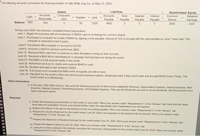

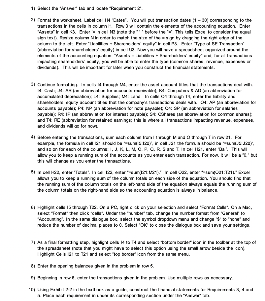
The following amounts summarize the financial position of Lite White Dog Inc. on May 31, 202x Cash Balance 1560 Accounts Receivable 600 Assets Computers (net) 0 + Supplies + Land - 60 7200 Liabilities Accounts Note Payable Payable 4800 0 Salaries Payable 0 Interest Payable 0 Shareholders' Equity Common Retained Shares Earnings 2400 2220 During June 202X the business completed these transactions: June 1: Began the business with an investment of $5400 cash in exchange for common shares June 1: Purchased a computer for a total of $4800 by signing a note payable Interest of 10% to be paid with the note payable on June 1 next year. The computer is expected to last 5 years June 5: Purchased office supples on account for $2700 June 9. Invoiced a clent for services performed, $900. June 13: Received $240 cash from a customer to clear the balance owing on their account June 20. Received a $800 ba for advertising for a campaign that had been run during the month June 23: Paid $900 of a bill received earlier in the month. June 25: Performed services for clients and received 55400 in cash June 30. Declared and paid a cash dividend of $360 June 30: A physical count revealed that $260 worth of supplies are still on hand. June 30. Paid $240 for the month's office rent and accrued employee salaries Employees work 5 days each work and are paid $2000 every Friday. The month onded on a Wednesday Other Information: 1) In the past, Leslie White Dog Inc. has used the following accounts on thorncome statement Revenue, Depreciation Exponse, Interest Expense, Rent Expenso Sataries Exponse, Advertising Expense and Supplies Expense. They use the Dividends account to record dividends. Not of accounts have been used each period Required: 28 89&&*&$ 1) Creato all necessary Jurnal entries for the month of June 202X. Place your answer under "Requirement in the "Answer" tab. Note that the dates have been pre-populated Ensure your journal entries match the appropriate date. Explanations are not requred 2) Analyze the effects of the above transactions on the accounting equation Place your answer under "Requirement in the 'Answer" tab a) Prepare the income Statement for the month ended June 30, 202X List expenses in decreasing order by amount Place your answer under Requirement in the "Answer tab 4) Prepare the Statement of Retained Earnings for the month ended June 30, 202x. Place your answer under "Requirement in the "Answer" tab. 5) Prepare the Balance Sheet at June 30, 202X. Place your answer under "Requirements in the Answer" tab. 5) Using the method outlined in the textbook ournal the necessary closing entries for the month ended June 30, 202X. Place your answer under "Requirement in the Answer tab 1) Select the "Answer" tab and locate "Requirement 2". 2) Format the worksheet. Label cell H4 "Dates". You will put transaction dates (1 - 30) corresponding to the transactions in the cells in column H. Row 3 will contain the elements of the accounting equation. Enter "Assets" in cell K3. Enter's in cell N3 (note the "T" before the "=". This tells Excel to consider the equal sign text). Resize column N in order to match the size of the = sign by dragging the right edge of the column to the left. Enter "Liabilities + Shareholders' equity" in cell P3. Enter "Type of SE Transaction" (abbreviation for shareholders' equity) in cell U3. Now you will have a spreadsheet organized around the elements of the accounting equation: "Assets = Liabilities + Shareholders' equity" and, for all transactions impacting shareholders' equity, you will be able to enter the type (common shares, revenue, expenses or dividends). This will be important for later when you construct the financial statements. 3) Continue formatting. In cells 14 through M4, enter the asset account titles that the transactions deal with. 14: Cash; J4: AR (an abbreviation for accounts receivable); K4: Computers & AD (an abbreviation for accumulated depreciation); L4: Supplies; M4: Land. In cells 04 through T4, enter the liability and shareholders' equity account titles that the company's transactions deals with. 04: AP (an abbreviation for accounts payable); P4: NP (an abbreviation for note payable); Q4: SP (an abbreviation for salaries payable); R4: IP (an abbreviation for interest payable); S4: CShares (an abbreviation for common shares); and T4: RE (abbreviation for retained earnings, this is where all transactions impacting revenue, expenses, and dividends will go for now). 4) Before entering the transactions, sum each column from I through M and Othrough Tin row 21. For example, the formula in cell 121 should be "=sum(15:120)", in cell J21 the formula should be "=sum(J5:J20)", and so on for each of the columns: I, J, K, L, M, O, P, Q, R, S and T. In cell H21, enter "Bal". This will allow you to keep a running sum of the accounts as you enter each transaction. For now, it will be a "0," but this will change as you enter the transactions. 5) In cell H22, enter "Totals". In cell 122, enter"=sum(121:M21)." In cell 022, enter"=sum(O21:T21)." Excel allows you to keep a running sum of the column totals on each side of the equation. You should find that the running sum of the column totals on the left-hand side of the equation always equals the running sum of the column totals on the right-hand side so the accounting equation is always in balance. 6) Highlight cells 15 through T22. On a PC, right click on your selection and select "Format Cells". On a Mac, select "Format" then click "cells". Under the "number" tab, change the number format from "General" to "Accounting". In the same dialogue box, select the symbol dropdown menu and change "$" to "none" and reduce the number of decimal places to 0. Select "OK" to close the dialogue box and save your settings. 7) As a final formatting step, highlight cells 14 to T4 and select "bottom border" icon in the toolbar at the top of the spreadsheet (note that you might have to select this option using the small arrow beside the icon). Highlight Cells 121 to T21 and select "top border" icon from the same menu. 8) Enter the opening balances given in the problem in row 5. 9) Beginning in row 6, enter the transactions given in the problem. Use multiple rows as necessary. 10) Using Exhibit 2-2 in the textbook as a guide, construct the financial statements for Requirements 3, 4 and 5. Place each requirement in under its corresponding section under the "Answer" tab