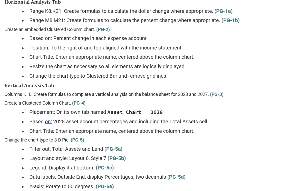
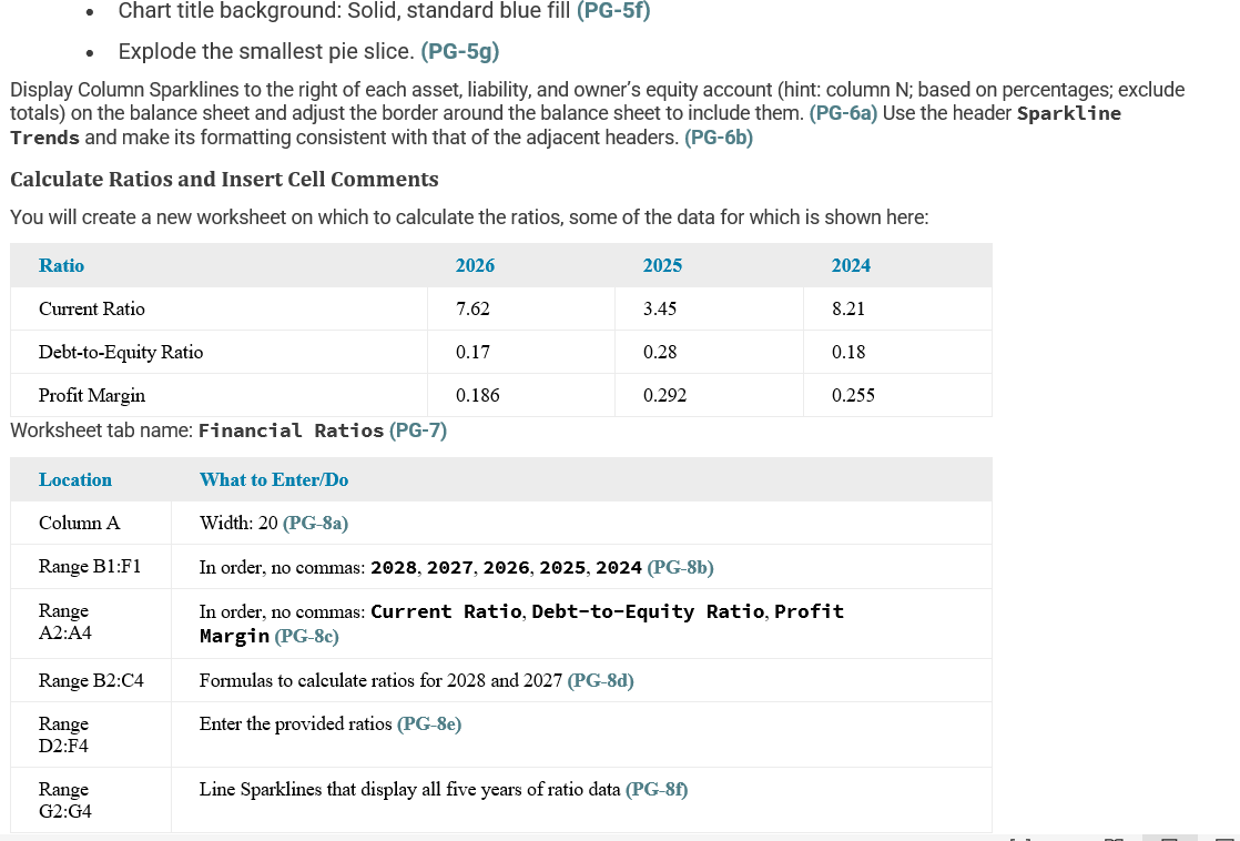
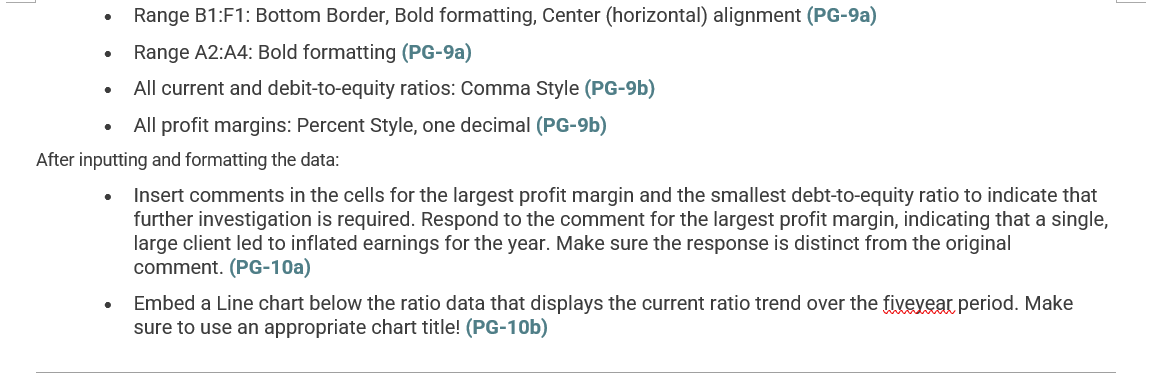
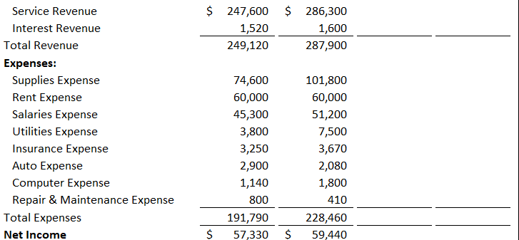
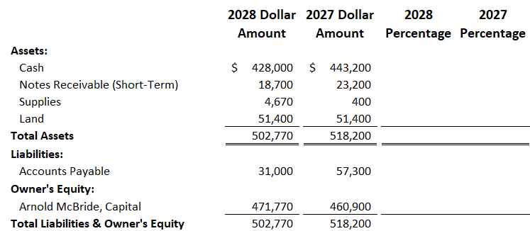
Horizontal Analysis Tab Range K8:K21: Create formulas to calculate the dollar change where appropriate. (PG-1a) Range M8:M21: Create formulas to calculate the percent change where appropriate. (PG-1b) Create an embedded Clustered Column chart. (PG-2) Based on: Percent change in each expense account Position: To the right of and top-aligned with the income statement Chart Title: Enter an appropriate name, centered above the column chart. Resize the chart as necessary so all elements are logically displayed. Change the chart type to Clustered Bar and remove gridlines. Vertical Analysis Tab Columns K-L: Create formulas to complete a vertical analysis on the balance sheet for 2028 and 2027. (PG-3) Create a Clustered Column Chart. (PG-4) Placement: On its own tab named Asset Chart - 2028 Based on: 2028 asset account percentages and including the Total Assets cell Chart Title: Enter an appropriate name, centered above the column chart. Change the chart type to 3-D Pie. (PG-5) Filter out: Total Assets and Land (PG-5a) Layout and style: Layout 6, Style 7 (PG-5b) Legend: Display it at bottom. (PG-5c) Data labels: Outside End; display Percentages, two decimals (PG-5d) Y-axis: Rotate to 50 degrees. (PG-5e) Chart title background: Solid, standard blue fill (PG-5f) Explode the smallest pie slice. (PG-5g) Display Column Sparklines to the right of each asset, liability, and owner's equity account (hint: column N; based on percentages; exclude totals) on the balance sheet and adjust the border around the balance sheet to include them. (PG-6a) Use the header Sparkline Trends and make its formatting consistent with that of the adjacent headers. (PG-6b) Calculate Ratios and Insert Cell Comments You will create a new worksheet on which to calculate the ratios, some of the data for which is shown here: Ratio 2026 2025 2024 Current Ratio 7.62 3.45 8.21 Debt-to-Equity Ratio 0.17 0.28 0.18 Profit Margin 0.186 0.292 0.255 Worksheet tab name: Financial Ratios (PG-7) Location What to Enter/Do Column A Width: 20 (PG-8a) Range B1:F1 In order, no commas: 2028, 2027, 2026, 2025, 2024 (PG-8b) Range A2:A4 In order, no commas: Current Ratio, Debt-to-Equity Ratio, Profit Margin (PG-8c) Range B2:C4 Formulas to calculate ratios for 2028 and 2027 (PG-8d) Range Enter the provided ratios (PG-8e) D2:F4 Line Sparklines that display all five years of ratio data (PG-8f) Range G2:G4 Range B1:F1: Bottom Border, Bold formatting, Center (horizontal) alignment (PG-9a) Range A2:A4: Bold formatting (PG-9a) All current and debit-to-equity ratios: Comma Style (PG-9b) All profit margins: Percent Style, one decimal (PG-9b) After inputting and formatting the data: Insert comments in the cells for the largest profit margin and the smallest debt-to-equity ratio to indicate that further investigation is required. Respond to the comment for the largest profit margin, indicating that a single, large client led to inflated earnings for the year. Make sure the response is distinct from the original comment. (PG-10a) Embed a Line chart below the ratio data that displays the current ratio trend over the fiveyear period. Make sure to use an appropriate chart title! (PG-10b) Service Revenue $ 247,600 $ 286,300 Interest Revenue 1,520 1,600 Total Revenue 249,120 287,900 Expenses: Supplies Expense 74,600 101,800 Rent Expense 60,000 60,000 Salaries Expense 45,300 51,200 Utilities Expense 3,800 7,500 Insurance Expense 3,250 3,670 Auto Expense 2,900 2,080 Computer Expense 1,140 1,800 Repair & Maintenance Expense 800 410 Total Expenses 191,790 228,460 Net Income 57,330 59,440 2028 Dollar 2027 Dollar 2028 2027 Amount Amount Percentage Percentage Assets: Cash $ 428,000 $ 443,200 Notes Receivable (Short-Term) 18,700 23,200 Supplies 4,670 400 Land 51,400 51,400 Total Assets 502,770 518,200 Liabilities: Accounts Payable 31,000 57,300 Owner's Equity: Arnold McBride, Capital 471,770 460,900 Total Liabilities & Owner's Equity 502,770 518,200 2028 Dollar 2027 Dollar 2028 2027 Amount Amount Percentage Percentage Assets: Cash $ 428,000 $ 443,200 Notes Receivable (Short-Term) 18,700 23,200 Supplies 4,670 400 Land 51,400 51,400 Total Assets 502,770 518,200 Liabilities: Accounts Payable 31,000 57,300 Owner's Equity: Arnold McBride, Capital 471,770 460,900 Total Liabilities & Owner's Equity 502,770 518,200