I am having issues with the formatting

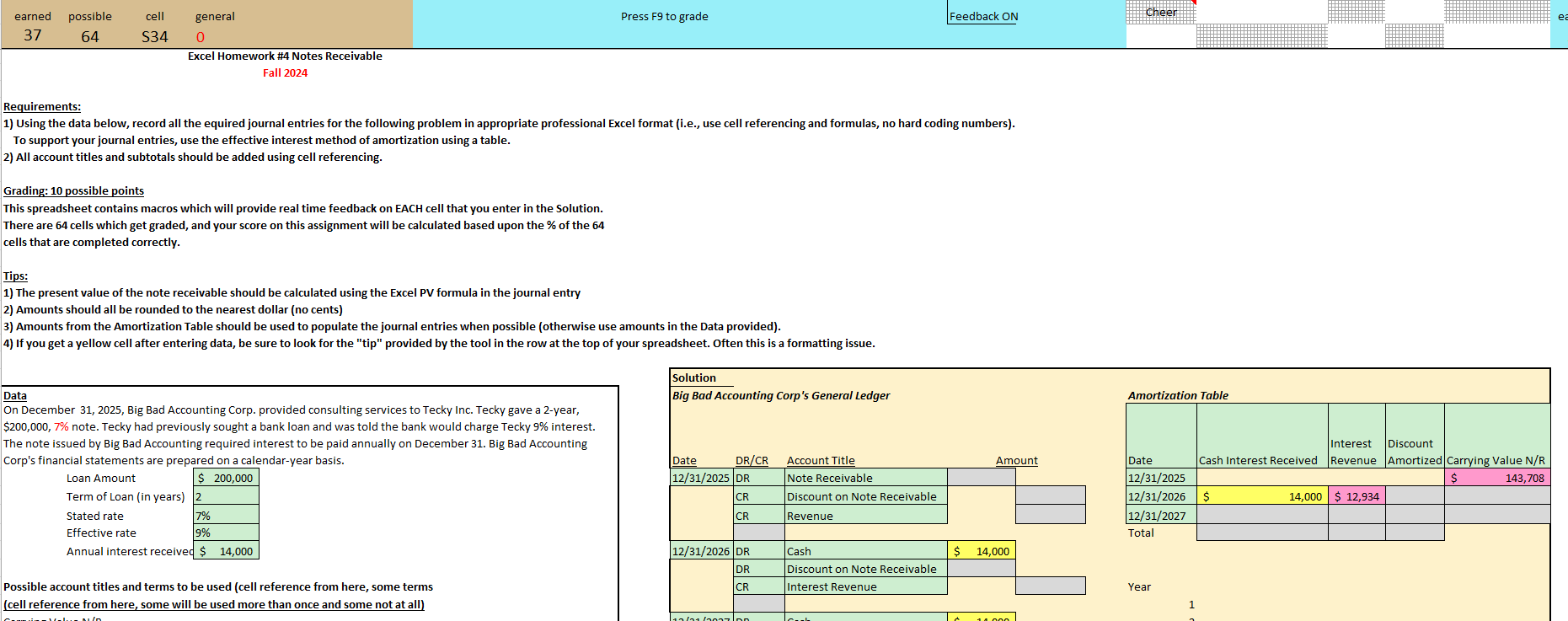
Using the data below, record all the required journal entries for the following problem in appropriate professional Excel format $($i$.$e$.,$ use cell referencing and formulas, no complex coding numbers$).$

To support your journal entries, use the effective interest method of amortization using a table.

All account titles and subtotals should be added using cell referencing.

Grading: $10$ possible points

This spreadsheet contains macros which will provide real time feedback on EACH cell that you enter in the Solution.

There are $64$ cells which get graded, and your score on this assignment will be calculated based upon the $\%$ of the $64$

cells that are completed correctly.

Tips:

The present value of the note receivable should be calculated using the Excel PV formula in the journal entry

Amounts should all be rounded to the nearest dollar $($no cents$)$

Amounts from the Amortization Table should be used to populate the journal entries when possible $($otherwise use amounts in the Data provided$).$

If you get a yellow cell after entering data, be sure to look for the "tip" provided by the tool in the row at the top of your spreadsheet. Often this is a formatting issue.

Data

On December $31,2025,$ Big Bad Accounting Corp. provided consulting services to Tecky Inc. Tecky gave a $2-$year,

$$200,000,7\%$ note. Tecky had previously sought a bank loan and was told the bank would charge Tecky $9\%$ interest.

ACTG$381$ Excel Homework #$4$ Notes Receivable Fall $2024$ Requirements: $1)$ Using the data below, record all the equired journal entries for the following problem in appropriate professional Excel format $($i$.$e$.,$ use cell referencing and formulas, no hard coding numbers$).$ To support your journal entries, use the effective interest method of amortization using a table. $2)$ All account titles and subtotals should be added using cell referencing.$$ Grading: $10$ possible points This spreadsheet contains macros which will provide real time feedback on EACH cell that you enter in the Solution.$$ There are $64$ cells which get graded, and your score on this assignment will be calculated based upon the $\%$ of the $64$ cells that are completed correctly. Tips: $1)$ The present value of the note receivable should be calculated using the Excel PV formula in the journal entry $2)$ Amounts should all be rounded to the nearest dollar $($no cents$)3)$ Amounts from the Amortization Table should be used to populate the journal entries when possible $($otherwise use amounts in the Data provided$).4)$ If you get a yellow cell after entering data, be sure to look for the "tip" provided by the tool in the row at the top of your spreadsheet. Often this is a formatting issue. Solution $$ Data $$ Big Bad Accounting Corp's General Ledger $$ Amortization Table $$ On December$31,2025,$ Big Bad Accounting Corp. provided consulting services to Tecky Inc. Tecky gave a $2-$year, $$200,000,7\%$ note. Tecky had previously sought a bank loan and was told the bank would charge Tecky $9\%$ interest. The note issued by Big Bad Accounting required interest to be paid annually on December $31.$ Big Bad Accounting Corp's financial statements are prepared on a calendar$-$year basis. Date DR$/$CR Account Title $$Amount$$ Loan Amount $$$$200,00012/31/2025$ DR Note Receivable $$$$143,708$ Term of Loan $($in years$)2$ CR Discount on Note Receivable $$ Stated rate $7\%$ CR Revenue $$ Effective rate $9\%$ Total $$ Annual interest received $$$$14,00012/31/2026$ DR Cash $$ DR Discount on Note Receivable $$ Possible account titles and terms to be used $($cell reference from here, some terms$$ CR Interest Revenue $($cell reference from here, some will be used more than once and some not at all$)$ Carrying Value N$/$R $12/31/2027$ DR Cash $$ Cash $$ DR Discount on Note Receivable $$ Cash Interest Received $$ CR Interest Revenue $$ CR $$ Date $$ DR Cash $$ Discount Amortized $$ CR Note Receivable $$ Discount on Note Receivable $$ DR $$ Interest Revenue $$ Note Receivable $$ Premium Amortized $$ Premium on Note Receivable $$ Revenue $$ Cash $$ To record revenue for consulting services and the receipt of the note $$ To record principal repayment $12/31/202512/31/202612/31/20272$ years $$$$200,0007\%9\%$