I have linearized dynamic bicycle model state space representation from Snider, Jarrod. $(2011).$Automatic Steering Methods for Autonomous Automobile Path Tracking. I am using Eq $29($attached$)$with error states. $4$ Path Tracking Control Using a Dynamic Model.

I want to modify this model. I will use states as lateral position error, lateral velocity error, longitunal position error, longitunal velocity error, yaw angle error and yaw rate error. My inputs are steering angle and longitunal velocity change $($dv$).$

Could you calculate new state space model?

Modelling the force genarated by the wheels as linearly proportionsl to the alip angle, the lateral forces are defined as

$F_{yf}=-c_f{}_f$

$F_{yr}=-c_r{}_r$

Annming a constant longitudinal valocity, $E_x^{}-0,$ allows the simplification

$F_{xf}=0$

Substituting Eqs. $21$ and $22$ into Eqz. $19$ and $20$ and soking for for $i_y$ and $r^{}$

$v_y^{}=\frac{-c_f[t{?}^{-1}(\frac{v_z+c_{gr}}{v_z})-]cos()-c_{r}t{?}^{-1}(\frac{v_r-l_{-r}}{v_e})}{m}-v_{z}r$

$r^{}=\frac{-l_f{c}_f[t{?}^{-1}(\frac{v_z+l_{f}r}{v_e})-]cos()+l_r{c}_{r}t{?}^{-1}(\frac{v_z-l_{z}r}{v_e})}{I_z}$

gives the dynamic bicycle model.

$4\mathrm{.}1\mathrm{.}1$ Limearized Dymamic Bicycle Model

To apply linear control mathods to the dynamic bicycle modal, the model must be linasrinad. Applying mall angle

assumptions to Eqz. $23$ and $24$ gives

$v_y^{}=\frac{-c_f{v}_y-c_f{l}_{f}r}{m{v}_x}+\frac{c_f}{m}+\frac{-c_r{v}_y+c_r{l}_{r}r}{m{v}_x}-v_{x}r$

$r^{}=\frac{-l_f{c}_f{v}_y-l_f^2{c}_{f}r}{I_x{v}_x}+\frac{l_f{c}_f}{I_x}+\frac{l_r{c}_r{v}_y-l_r^2{c}_{r}r}{I_x{v}_x}$

Collacting torms results in

$v_y^{}=\frac{-(c_{}+c_r)}{m{v}_x}{v}_y+[\frac{(l_r{c}_r-l_{}{c}_f)}{m{E}_x}-v_x]r+\frac{c_{}}{m}$

$r^{}=\frac{l_r{c}_r-l_f{c}_f}{I_x{v}_x}{v}_y+\frac{-(l_f^2{c}_f+l_r{c}_r)}{I_x{v}_x}r+\frac{{}_f{c}_{}}{m}$ Finally, the linasr dyuamic bicycle model can be writtan in state space form as

$4\mathrm{.}1\mathrm{.}2$ Path Coordinates

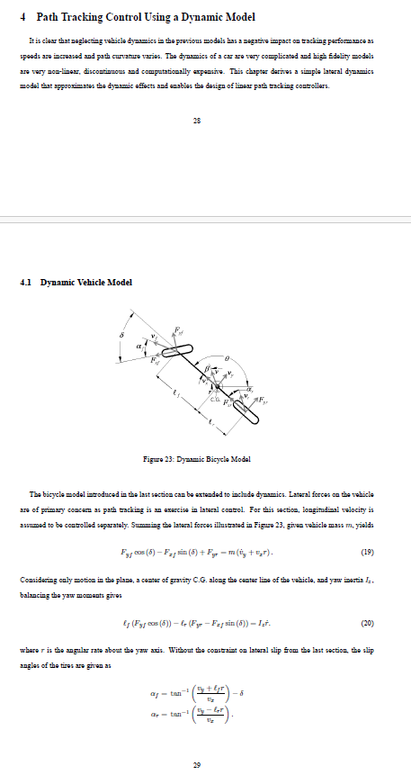
Figure $24$: Dyzamic Bicycle Modal in path coordinates

As with the kinematic bicycle modal, it is usafal to axprass the dynamic bicycle model with respact to the path.

With the constant longitudinal valocity asnumption, the yaw rate derived from the path $r(a)$ is definad as

$r(s)=(s)v_{x^{-}}$

Path derived lataral acceleration iy $($s$)$ follow: as

$t_y^{}(s)-(s)v_{x^{*}}^2$

Letting $c_{eg}$ be the orthogonal distance of the C$.$G$.$ to the path,

vec$(e{)}_{ag}=(v_y^{}+v_{x}r)-v_y^{}(s)$

$=v_y^{}+v_x(r-r(s))$

$=v_y^{}+v_x{}_a^{}$ and

${}_{zg}^{}-v_y+v_{z}sin({}_z)$

where ${}_a$ was provioualy dafined as $-{}_p(s).$ Subatituting $(c_{eg},{}_p)$ into Eqs. $25$ and $26$ yields

$e_{cg}^{}-v_z{}_n^{}=\frac{-(c_f+c_r)}{ma{}_x}(c_{ng}^{}-v_x{}_n)$

$+[\frac{l_r{C}_r-l_f{C}_f}{m{E}_x}-v_x]({}_e^{}+r(s))+\frac{c_f}{m}$

$e_{cg}^{}=\frac{-(c_f+c_r)}{m{v}_x}{c}_{cg}^{}+\frac{c_f+c_r}{m}{}_a$

$+\frac{l_r{c}_r-l_f{c}_l}{m{v}_x}{}_e^{}+[\frac{l_r{c}_r-l_f{c}_f}{m{v}_x}-v_x]r(s)+\frac{c_f}{m}$

vec$({)}_e+r^{}(s)=\frac{l_r{c}_r-l_r{c}_f}{I_x{v}_x}(c_{eg}^{}-v_x{}_n)$

$+\frac{-({}_f^{{}_f}{c}_J+{}_r^2{c}_r)}{I_z{v}_z}({}_n^{}+r(s))+\frac{{}_f{c}_f}{m}\frac{?}{b}$

$ar({)}_n=\frac{l_r{B}_r-l_f{c}_f}{I_z{v}_x}{c}_{cg}^{}+\frac{l_f{c}_f-l_r{c}_r}{I_z}{}_n$

$+\frac{-(l_f^2{c}_f+l_r^2{c}_r)}{I_x{v}_x}({}_n^{}+r(s))+\frac{l_f{c}_f}{m}-r^{}(s).$

The state space model in tracking error variables is tharafore given by

$32$