

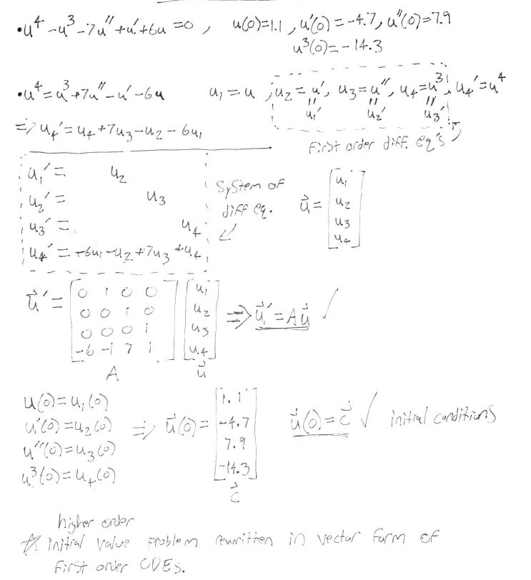
Question: I have rewritten the higher order initial value problem to a system of first-order ODEs as you can see below, I just need you to
I have rewritten the higher order initial value problem to a system of first-order ODEs as you can see below, I just need you to do part B now and show me how you would code it. Below I have also put some code for another problem which was for euler implicit method and third order runge-kutta method, however I think my implicit euler is actually explicit I just dont know how to use the code for this problem
PLEASE DO NOT USE any built-in Matlab functions for solving ODEs such as ode23 or ode45.
Thank you so much, I will upvote.
%% EULER IMPLICIT METHOD
h = 0.1; x0 = 0; u0 = 1; x_end = 2; x(1)=x0; u(1)=u0; %number of steps n = (x_end-x0)/h;
for k=1:n uprime(k+1) = -x(k)*u(k) + exp(-(x(k)^2)/2); x(k+1) = x(k) + h; u(k+1) = u(k) + uprime(k+1)*h; end
%transpose x and u into column vectors xvalues = x'; uvalues = u';
%% THIRD ORDER RANGE KUTTA METHOD
h = 0.1; x0 = 0; u0 = 1; x_end = 2; x1(1)=x0; u1(1)=u0; x1= 0:h:2; y1= zeros(1,length(x1)); F = @(x,u) -x.*u + exp(-(x.^2)/2); for i=1:(length(x1)-1) k1 = F(x1(i),u1(i)); k2 = F(x1(i)+0.5*h,u1(i)+k1); k3 = F((x1(i)+0.5*h),(u1(i)-k1+2*k2)); u1(i+1) = u1(i) + (1/6)*(k1+4*k2+k3)*h; end u1values = u1';
%% PLOT ALL THREE GRAPHS
exact = @(x) exp(-(x.^2)/2).*(x+1); plot(x,u, '--b'); xlim([0 2]) hold on fplot(exact,[x0,x_end], 'r'); hold on plot(x1,u1, '--g'); legend('euler','exact','runge-kutta')
step = xvalues; implicit = uvalues; RungeKutta = u1values; exact = exact(xvalues); table(step,implicit,RungeKutta,exact)
Consider the following initial value problem for uCx) defined on x0 u , , , ,-u , , , _ 7 u , , + u , + 6 u 0 , ("prime" is the derivative, d/dx) n(0) = 1.1 , u'(0) = _ 4.7 , 11"(0) = 7.9 , 11"(0) =-14.3 (a) Find the analytic solution, which will be used to validate the numerical solutions. (b) Solve the initial value problem by first converting the original system into a system of first-order ODEs, then solving the latter using the following three methods ("Ar" is "h" in the textbook): (I) Euler's explicit method, with ?x = 0.1 II) Euler's explicit method, with Ax 0.03 TII) Mid-point method, with Ax-0.1 In all 3 cases, numerically integrate the system to x 1.5 to find the solution over the interval of 0 x 1.5. Plot the analytic solution and the numerical solutions using methods (, (II), and (III) over the interval of 0Sx 1.5. Collect all four curves in one plot and clearly label the curves. Consider the following initial value problem for uCx) defined on x0 u , , , ,-u , , , _ 7 u , , + u , + 6 u 0 , ("prime" is the derivative, d/dx) n(0) = 1.1 , u'(0) = _ 4.7 , 11"(0) = 7.9 , 11"(0) =-14.3 (a) Find the analytic solution, which will be used to validate the numerical solutions. (b) Solve the initial value problem by first converting the original system into a system of first-order ODEs, then solving the latter using the following three methods ("Ar" is "h" in the textbook): (I) Euler's explicit method, with ?x = 0.1 II) Euler's explicit method, with Ax 0.03 TII) Mid-point method, with Ax-0.1 In all 3 cases, numerically integrate the system to x 1.5 to find the solution over the interval of 0 x 1.5. Plot the analytic solution and the numerical solutions using methods (, (II), and (III) over the interval of 0Sx 1.5. Collect all four curves in one plot and clearly label the curves
Step by Step Solution
There are 3 Steps involved in it

Get step-by-step solutions from verified subject matter experts