I need help with this excel spreadsheet

#7,10,11,12,13

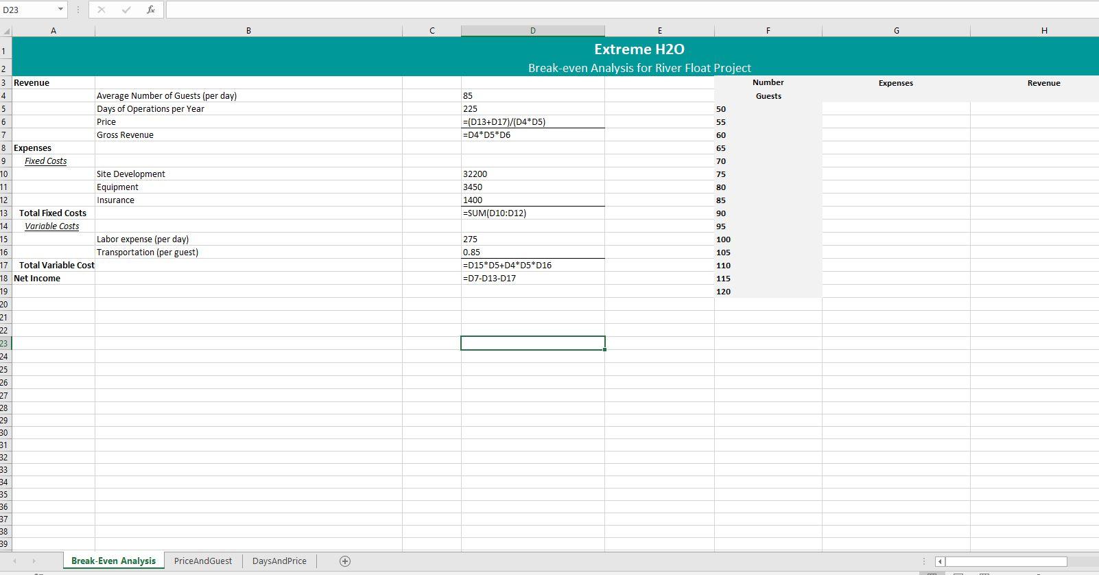
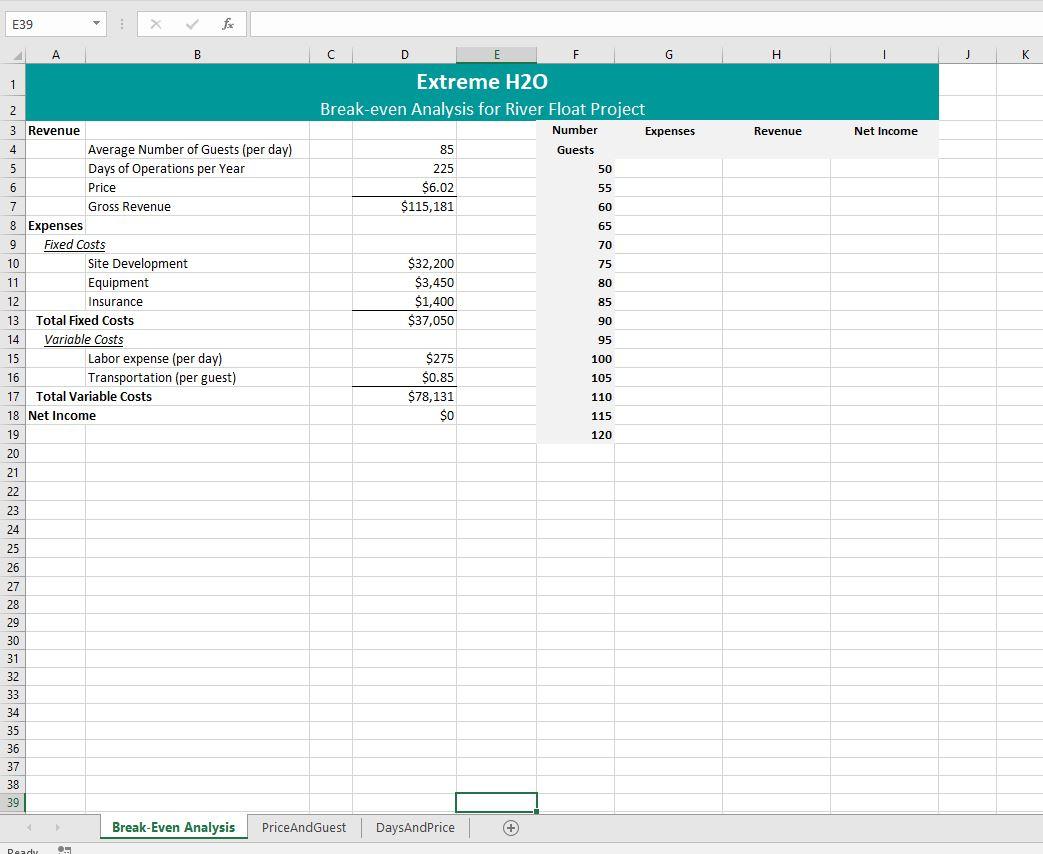
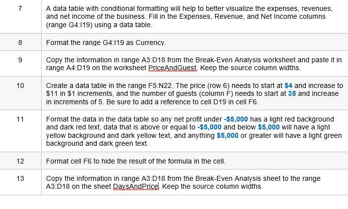
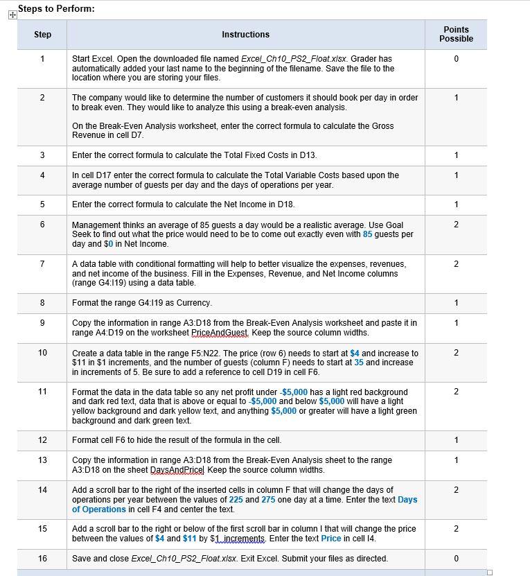
7	A data table with conditional formatting will help to better visualize the expenses, revenues, and net income of the business. Fill in the Expenses, Revenue, and Net Income columns (range G4:I19) using a data table.
8	Format the range G4:I19 as Currency.
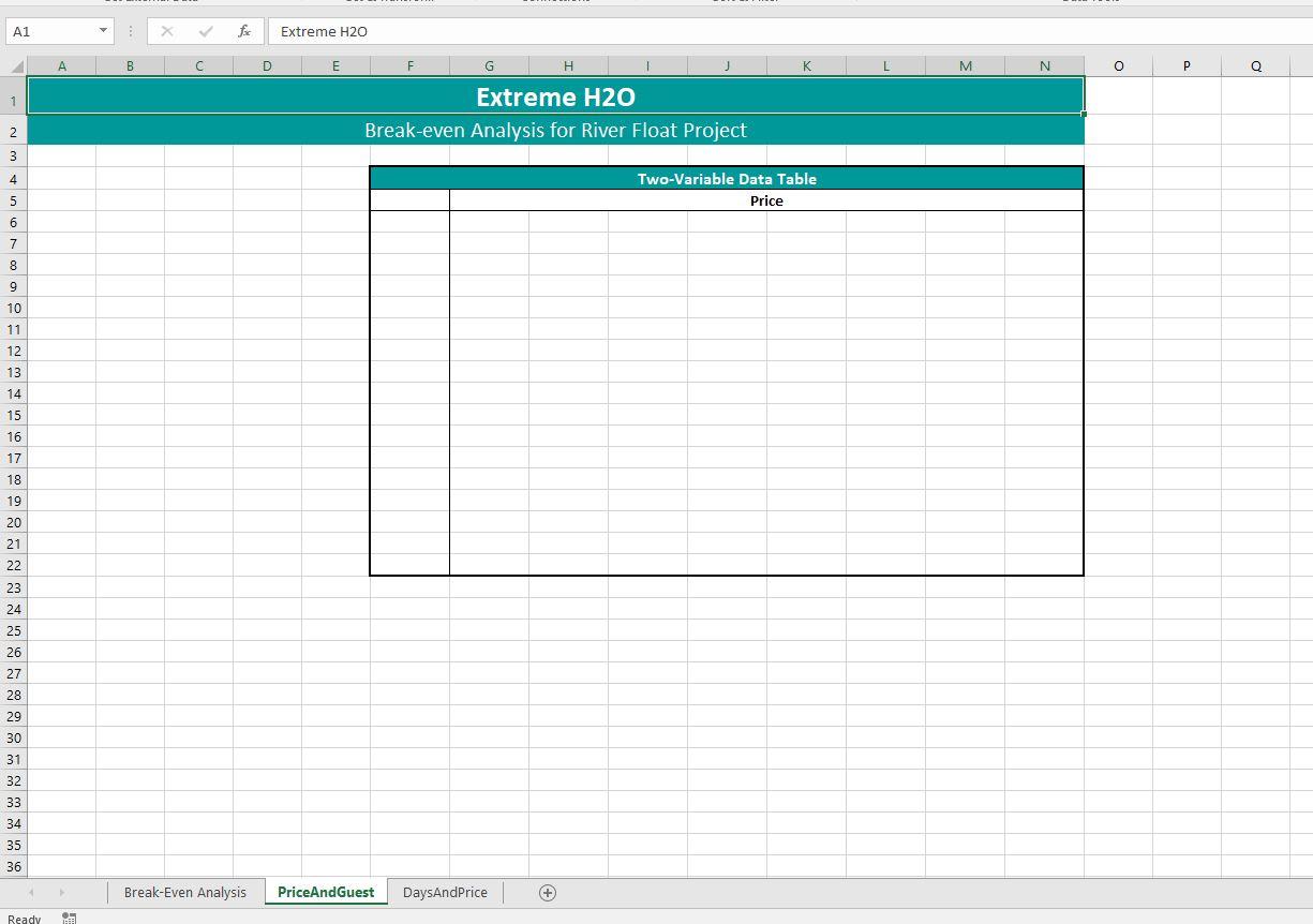
9	Copy the information in range A3:D18 from the Break-Even Analysis worksheet and paste it in range A4:D19 on the worksheet PriceAndGuest. Keep the source column widths.
10	Create a data table in the range F5:N22. The price (row 6) needs to start at $4 and increase to $11 in $1 increments, and the number of guests (column F) needs to start at 35 and increase in increments of 5. Be sure to add a reference to cell D19 in cell F6.
11	Format the data in the data table so any net profit under -$5,000 has a light red background and dark red text, data that is above or equal to -$5,000 and below $5,000 will have a light yellow background and dark yellow text, and anything $5,000 or greater will have a light green background and dark green text.
12	Format cell F6 to hide the result of the formula in the cell.
13	Copy the information in range A3:D18 from the Break-Even Analysis sheet to the range A3:D18 on the sheet DaysAndPrice. Keep the source column widths.

D23 B H 1 D E F Extreme H20 Break-even Analysis for River Float Project Number 85 Guests 225 50 =(D13+D17)/(D4*D5) 55 =D4*D5*D6 Expenses Revenue Revenue 60 65 70 75 80 32200 3450 1400 =SUM(D10:012) 85 90 95 2 3 Revenue 4 Average Number of Guests (per day) 5 Days of Operations per Year 6 Price 7 Gross Revenue 8 Expenses 9 Fixed Costs 70 Site Development 11 Equipment 12 Insurance 13 Total Fixed Costs 14 Variable costs 15 Labor expense (per day) 76 Transportation (per guest) 17 Total Variable Cost 78 Net Income 19 20 21 22 23 24 25 26 27 275 0.85 =D15*D5+D4*D5*D16 =D7-D13-D17 100 105 110 115 120 28 29 30 31 32 33 34 35 36 37 38 39 Break-Even Analysis PriceAndGuest DaysAndPrice + M E39 X A B G H J K 1 2 Revenue Net Income D E F Extreme H20 Break-even Analysis for River Float Project Number Expenses 85 Guests 225 50 $6.02 $115,181 65 55 60 70 75 3 Revenue 4 Average Number of Guests (per day) 5 Days of Operations per Year 6 Price 7 Gross Revenue 8 Expenses 9 Fixed Costs 10 Site Development 11 Equipment 12 Insurance 13 Total Fixed Costs 14 Variable Costs 15 Labor expense (per day) 16 Transportation (per guest) 17 Total Variable Costs 18 Net Income 80 $32,200 $3,450 $1,400 $37,050 85 90 95 100 105 $275 $0.85 $78,131 $0 110 115 120 19 20 21 22 23 24 25 26 27 28 29 30 31 32 33 34 35 36 37 38 39 Break-Even Analysis PriceAndGuest DaysAndPrice + Ready A1 X fc Extreme H20 A B C D E G H K M N 0 P Q 1 Extreme H20 Break-even Analysis for River Float Project 2 3 4 Two-Variable Data Table Price 5 6 7 8 9 10 11 12 13 14 15 16 17 18 19 20 21 22 23 24 25 26 27 28 29 30 31 32 33 34 35 36 Break-Even Analysis PriceAndGuest DaysAndPrice (+ Ready THARI A1 Extreme H20 B D E G H J K L M N O 1 1 Extreme H20 Break-even Analysis for River Float Project 2 3 4 5 6 7 8 8 9 10 11 12 13 14 15 16 17 18 19 20 21 22 23 24 25 26 27 28 29 30 31 32 33 34 35 23 + Break-Even Analysis PriceAndGuest DaysAndPrice + Ready A data table with conditional formatting will help to better visualize the expenses, revenues, and net income of the business. Fill in the Expenses, Revenue, and Net Income columns (range G4:119) using a data table. 8 Format the range G4:119 as Currency. Copy the information in range A3:D18 from the Break-Even Analysis worksheet and paste it in range A4:D19 on the worksheet PriceAndGuest. Keep the source column widths. 9 10 Create a data table in the range F5:N22. The price (row 6) needs to start at $4 and increase to $11 in $1 increments, and the number of guests (column F) needs to start at 35 and increase in increments of 5. Be sure to add a reference to cell D19 in cell F6. 11 Format the data in the data table so any net profit under $5,000 has a light red background and dark red text, data that is above or equal to -$5,000 and below $5,000 will have a light yellow background and dark yellow text, and anything $5,000 or greater will have a light green background and dark green text. 12 Format cell F6 to hide the result of the formula in the cell. 13 Copy the information in range A3:D18 from the Break-Even Analysis sheet to the range A3:D18 on the sheet DaysAndPricel Keep the source column widths. Steps to Perform: Step Instructions Points Possible 1 0 2 1 3 1 4 1 5 1 6 2 7 2 8 1 Start Excel. Open the downloaded file named Excel_Ch10_PS2_Float.xlsx. Grader has automatically added your last name to the beginning of the filename. Save the file to the location where you are storing your files. The company would like to determine the number of customers it should book per day in order to break even. They would like to analyze this using a break-even analysis. On the Break-Even Analysis worksheet, enter the correct formula to calculate the Gross Revenue in cell D7 Enter the correct formula to calculate the Total Fixed Costs in D13. In cell D17 enter the correct formula to calculate the Total Variable Costs based upon the average number of guests per day and the days of operations per year. Enter the correct formula to calculate the Net Income in D18. Management thinks an average of 85 guests a day would be a realistic average. Use Goal Seek to find out what the price would need to be to come out exactly even with 85 guests per day and $0 in Net Income. A data table with conditional formatting will help to better visualize the expenses, revenues, and net income of the business. Fill in the Expenses, Revenue, and Net Income columns (range G4:119) using a data table, Format the range G4:119 as Currency. Copy the information in range A3:D18 from the Break-Even Analysis worksheet and paste it in range A4:D19 on the worksheet PriceAndGuest. Keep the source column widths. Create a data table in the range F5:N22. The price (row 6) needs to start at $4 and increase to $11 in $1 increments, and the number of guests (column F) needs to start at 35 and increase in increments of 5. Be sure to add a reference to cell D19 in cell F6. Format the data in the data table so any net profit under $5,000 has a light red background and dark red text, data that is above or equal to $5,000 and below $5,000 will have a light yellow background and dark yellow text, and anything $5,000 or greater will have a light green background and dark green text. Format cell F6 to hide the result of the formula in the cell. Copy the information in range A3:D18 from the Break-Even Analysis sheet to the range A3:D18 on the sheet DaysAndPrice! Keep the source column widths. Add a scroll bar to the right of the inserted cells in column F that will change the days of operations per year between the values of 225 and 275 one day at a time. Enter the text Days of Operations in cell F4 and center the text. Add a scroll bar to the right or below of the first scroll bar in column I that will change the price between the values of $4 and $11 by $1 increments. Enter the text Price in cell 14. Save and close Excel_Ch10_PS2_Float.xlsx. Exit Excel. Submit your files as directed. 9 1 10 2 11 2 12 1 13 1 14 2 15 2 16 0 D23 B H 1 D E F Extreme H20 Break-even Analysis for River Float Project Number 85 Guests 225 50 =(D13+D17)/(D4*D5) 55 =D4*D5*D6 Expenses Revenue Revenue 60 65 70 75 80 32200 3450 1400 =SUM(D10:012) 85 90 95 2 3 Revenue 4 Average Number of Guests (per day) 5 Days of Operations per Year 6 Price 7 Gross Revenue 8 Expenses 9 Fixed Costs 70 Site Development 11 Equipment 12 Insurance 13 Total Fixed Costs 14 Variable costs 15 Labor expense (per day) 76 Transportation (per guest) 17 Total Variable Cost 78 Net Income 19 20 21 22 23 24 25 26 27 275 0.85 =D15*D5+D4*D5*D16 =D7-D13-D17 100 105 110 115 120 28 29 30 31 32 33 34 35 36 37 38 39 Break-Even Analysis PriceAndGuest DaysAndPrice + M E39 X A B G H J K 1 2 Revenue Net Income D E F Extreme H20 Break-even Analysis for River Float Project Number Expenses 85 Guests 225 50 $6.02 $115,181 65 55 60 70 75 3 Revenue 4 Average Number of Guests (per day) 5 Days of Operations per Year 6 Price 7 Gross Revenue 8 Expenses 9 Fixed Costs 10 Site Development 11 Equipment 12 Insurance 13 Total Fixed Costs 14 Variable Costs 15 Labor expense (per day) 16 Transportation (per guest) 17 Total Variable Costs 18 Net Income 80 $32,200 $3,450 $1,400 $37,050 85 90 95 100 105 $275 $0.85 $78,131 $0 110 115 120 19 20 21 22 23 24 25 26 27 28 29 30 31 32 33 34 35 36 37 38 39 Break-Even Analysis PriceAndGuest DaysAndPrice + Ready A1 X fc Extreme H20 A B C D E G H K M N 0 P Q 1 Extreme H20 Break-even Analysis for River Float Project 2 3 4 Two-Variable Data Table Price 5 6 7 8 9 10 11 12 13 14 15 16 17 18 19 20 21 22 23 24 25 26 27 28 29 30 31 32 33 34 35 36 Break-Even Analysis PriceAndGuest DaysAndPrice (+ Ready THARI A1 Extreme H20 B D E G H J K L M N O 1 1 Extreme H20 Break-even Analysis for River Float Project 2 3 4 5 6 7 8 8 9 10 11 12 13 14 15 16 17 18 19 20 21 22 23 24 25 26 27 28 29 30 31 32 33 34 35 23 + Break-Even Analysis PriceAndGuest DaysAndPrice + Ready A data table with conditional formatting will help to better visualize the expenses, revenues, and net income of the business. Fill in the Expenses, Revenue, and Net Income columns (range G4:119) using a data table. 8 Format the range G4:119 as Currency. Copy the information in range A3:D18 from the Break-Even Analysis worksheet and paste it in range A4:D19 on the worksheet PriceAndGuest. Keep the source column widths. 9 10 Create a data table in the range F5:N22. The price (row 6) needs to start at $4 and increase to $11 in $1 increments, and the number of guests (column F) needs to start at 35 and increase in increments of 5. Be sure to add a reference to cell D19 in cell F6. 11 Format the data in the data table so any net profit under $5,000 has a light red background and dark red text, data that is above or equal to -$5,000 and below $5,000 will have a light yellow background and dark yellow text, and anything $5,000 or greater will have a light green background and dark green text. 12 Format cell F6 to hide the result of the formula in the cell. 13 Copy the information in range A3:D18 from the Break-Even Analysis sheet to the range A3:D18 on the sheet DaysAndPricel Keep the source column widths. Steps to Perform: Step Instructions Points Possible 1 0 2 1 3 1 4 1 5 1 6 2 7 2 8 1 Start Excel. Open the downloaded file named Excel_Ch10_PS2_Float.xlsx. Grader has automatically added your last name to the beginning of the filename. Save the file to the location where you are storing your files. The company would like to determine the number of customers it should book per day in order to break even. They would like to analyze this using a break-even analysis. On the Break-Even Analysis worksheet, enter the correct formula to calculate the Gross Revenue in cell D7 Enter the correct formula to calculate the Total Fixed Costs in D13. In cell D17 enter the correct formula to calculate the Total Variable Costs based upon the average number of guests per day and the days of operations per year. Enter the correct formula to calculate the Net Income in D18. Management thinks an average of 85 guests a day would be a realistic average. Use Goal Seek to find out what the price would need to be to come out exactly even with 85 guests per day and $0 in Net Income. A data table with conditional formatting will help to better visualize the expenses, revenues, and net income of the business. Fill in the Expenses, Revenue, and Net Income columns (range G4:119) using a data table, Format the range G4:119 as Currency. Copy the information in range A3:D18 from the Break-Even Analysis worksheet and paste it in range A4:D19 on the worksheet PriceAndGuest. Keep the source column widths. Create a data table in the range F5:N22. The price (row 6) needs to start at $4 and increase to $11 in $1 increments, and the number of guests (column F) needs to start at 35 and increase in increments of 5. Be sure to add a reference to cell D19 in cell F6. Format the data in the data table so any net profit under $5,000 has a light red background and dark red text, data that is above or equal to $5,000 and below $5,000 will have a light yellow background and dark yellow text, and anything $5,000 or greater will have a light green background and dark green text. Format cell F6 to hide the result of the formula in the cell. Copy the information in range A3:D18 from the Break-Even Analysis sheet to the range A3:D18 on the sheet DaysAndPrice! Keep the source column widths. Add a scroll bar to the right of the inserted cells in column F that will change the days of operations per year between the values of 225 and 275 one day at a time. Enter the text Days of Operations in cell F4 and center the text. Add a scroll bar to the right or below of the first scroll bar in column I that will change the price between the values of $4 and $11 by $1 increments. Enter the text Price in cell 14. Save and close Excel_Ch10_PS2_Float.xlsx. Exit Excel. Submit your files as directed. 9 1 10 2 11 2 12 1 13 1 14 2 15 2 16 0