I will vote your Answer Definitely please give me Right answer of my question

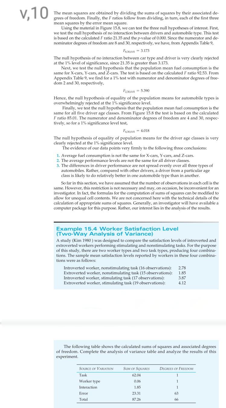
V, 10 The mean squares are obtained by dividing the sums of squares by their associated de- grees of freedom. Finally, the F ratios follow from dividing, in turn, each of the first three mean squares by the error mean square. Using the material in Figure 15.8, we can test the three null hypotheses of interest. First, we test the null hypothesis of no interaction between drivers and automobile type. This test is based on the calculated F ratio 21.35 and the p-value of 0.000. Since the numerator and de- nominator degrees of freedom are 8 and 30, respectively, we have, from Appendix Table 9, F9,30,001 = 3.173 The null hypothesis of no interaction between car type and driver is very clearly rejected at the 1% level of significance, since 21.35 is greater than 3.173. Next, we test the null hypothesis that the population mean fuel consumption is the same for X-cars, Y-cars, and Z-cars. The test is based on the calculated F ratio 92.53. From Appendix Table 9, we find for a 1% test with numerator and denominator degrees of free- dom 2 and 30, respectively, F2,30,001 = 5.390 Hence, the null hypothesis of equality of the population means for automobile types is overwhelmingly rejected at the 1% significance level. Finally, we test the null hypothesis that the population mean fuel consumption is the same for all five driver age classes. From Figure 15.8 the test is based on the calculated F ratio 85.01. The numerator and denominator degrees of freedom are 4 and 30, respec- tively, so for a 1% significance level test, F4,30,000 = 4.018 The null hypothesis of equality of population means for the driver age classes is very clearly rejected at the 1% significance level. The evidence of our data points very firmly to the following three conclusions: 1. Average fuel consumption is not the same for X-cars, Y-cars, and Z-cars. 2. The average performance levels are not the same for all driver classes. 3. The differences in driver performance are not spread evenly over all three types of automobiles. Rather, compared with other drivers, a driver from a particular age class is likely to do relatively better in one automobile type than in another. So far in this section, we have assumed that the number of observations in each cell is the same. However, this restriction is not necessary and may, on occasion, be inconvenient for an investigator. In fact, the formulas for the computation of sums of squares can be modified to allow for unequal cell contents. We are not concerned here with the technical details of the calculation of appropriate sums of squares. Generally, an investigator will have available a computer package for this purpose. Rather, our interest lies in the analysis of the results. Example 15.4 Worker Satisfaction Level (Two-Way Analysis of Variance) A study (Kim 1980 ) was designed to compare the satisfaction levels of introverted and extroverted workers performing stimulating and nonstimulating tasks. For the purpose of this study, there are two worker types and two task types, producing four combina- tions. The sample mean satisfaction levels reported by workers in these four combina- tions were as follows: Introverted worker, nonstimulating task (16 observations): Extroverted worker, nonstimulating task (15 observations): Introverted worker, stimulating task (17 observations): Extroverted worker, stimulating task (19 observations): 2.78 1.85 3.87 4.12 The following table shows the calculated sums of squares and associated degrees of freedom. Complete the analysis of variance table and analyze the results of this experiment. SOURCE OF VARIATION SUM OF SQUARES DEGREES OF FREEDOM Task 62.04 1 Worker type 0.06 1 Interaction 1.85 1 Error 23.31 63 Total 87.26 66