Illustrated Excel $2019|$ Module $8$: SAM Project $1$a

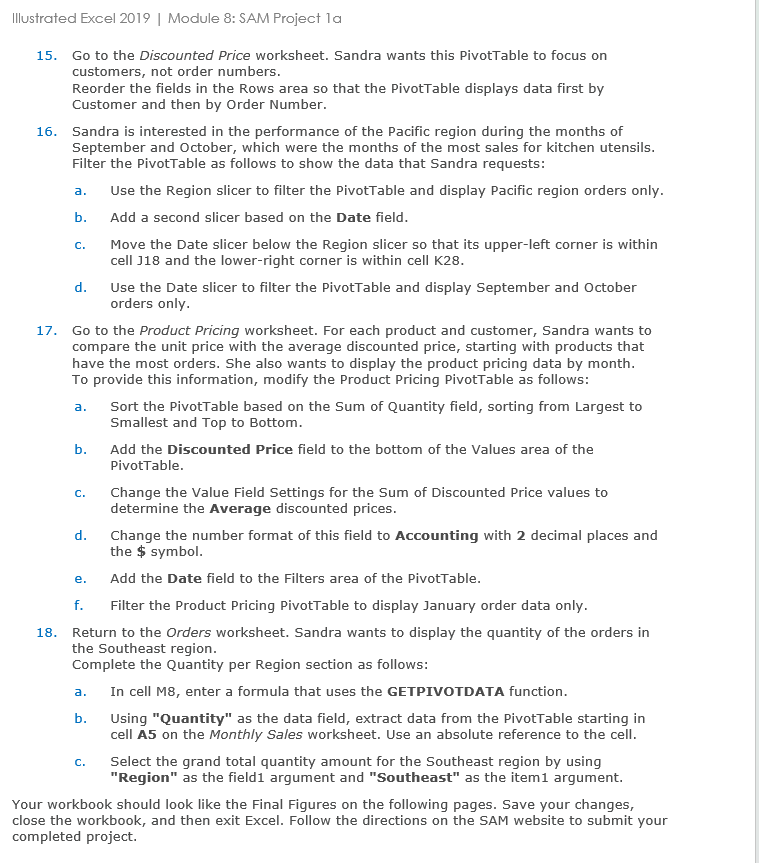
$15.$ Go to the Discounted Price worksheet. Sandra wants this PivotTable to focus on customers, not order numbers.

Reorder the fields in the Rows area so that the PivotTable displays data first by Customer and then by Order Number.

$16.$ Sandra is interested in the performance of the Pacific region during the months of September and October, which were the months of the most sales for kitchen utensils. Filter the PivotTable as follows to show the data that Sandra requests:

a$.$ Use the Region slicer to filter the PivotTable and display Pacific region orders only.

b$.$ Add a second slicer based on the Date field.

c$.$ Move the Date slicer below the Region slicer so that its upper$-$left corner is within cell J$18$ and the lower$-$right corner is within cell K$28.$

d$.$ Use the Date slicer to filter the PivotTable and display September and October orders only.

$17.$ Go to the Product Pricing worksheet. For each product and customer, Sandra wants to compare the unit price with the average discounted price, starting with products that have the most orders. She also wants to display the product pricing data by month. To provide this information, modify the Product Pricing PivotTable as follows:

a$.$ Sort the PivotTable based on the Sum of Quantity field, sorting from Largest to Smallest and Top to Bottom.

b$.$ Add the Discounted Price field to the bottom of the Values area of the PivotTable.

c$.$ Change the Value Field Settings for the Sum of Discounted Price values to determine the Average discounted prices.

d$.$ Change the number format of this field to Accounting with $2$ decimal places and the $\backslash$$ symbol.

e$.$ Add the Date field to the Filters area of the PivotTable.

f$.$ Filter the Product Pricing PivotTable to display January order data only.

$18.$ Return to the Orders worksheet. Sandra wants to display the quantity of the orders in the Southeast region.

Complete the Quantity per Region section as follows:

a$.$ In cell M$8,$ enter a formula that uses the GETPIVOTDATA function.

b$.$ Using "Quantity" as the data field, extract data from the PivotTable starting in cell A$5$ on the Monthly Sales worksheet. Use an absolute reference to the cell.

c$.$ Select the grand total quantity amount for the Southeast region by using "Region" as the field$1$ argument and "Southeast" as the item$1$ argument.

Your workbook should look like the Final Figures on the following pages. Save your changes, close the workbook, and then exit Excel. Follow the directions on the SAM website to submit your completed project.