Instructions

Background

Question 1 problem. Please help me with this.

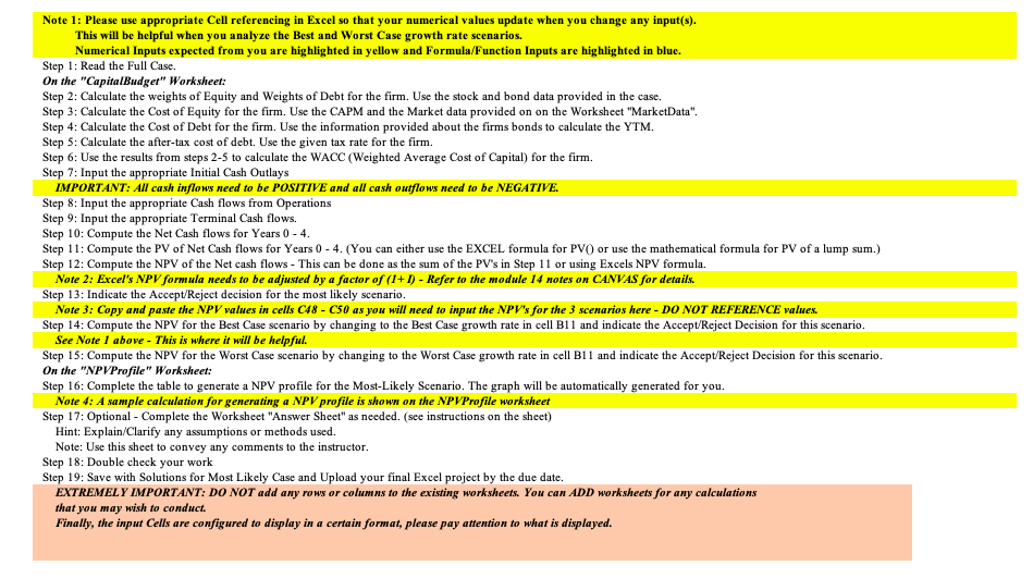
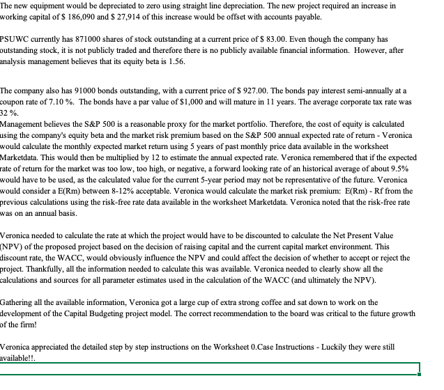
Note 1: Please use appropriate Cell referencing in Excel so that your numerical values update when you change any input(s). This will be helpful when you analyze the Best and Worst Case growth rate scenarios. Numerical Inputs expected from you are highlighted in yellow and Formula/Function Inputs are highlighted in blue. Step 1: Read the Full Case. On the "CapitalBudget" Worksheet: Step 2: Calculate the weights of Equity and Weights of Debt for the firm. Use the stock and bond data provided in the case. Step 3: Calculate the Cost of Equity for the firm. Use the CAPM and the Market data provided on on the Worksheet "MarketData". Step 4: Calculate the Cost of Debt for the firm. Use the information provided about the firms bonds to calculate the YTM. Step 5: Calculate the after-tax cost of debt. Use the given tax rate for the firm. Step 6: Use the results from steps 2-5 to calculate the WACC (Weighted Average Cost of Capital) for the firm. Step 7: Input the appropriate Initial Cash Outlays IMPORTANT: All cash inflows need to be POSITIVE and all cash outflows need to be NEGATIVE. Step 8: Input the appropriate Cash flows from Operations Step 9: Input the appropriate Terminal Cash flows. Step 10: Compute the Net Cash flows for Years 0 - 4. Step 11: Compute the PV of Net Cash flows for Years 0 - 4. (You can either use the EXCEL formula for PV() or use the mathematical formula for PV of a lump sum.) Step 12: Compute the NPV of the Net cash flows - This can be done as the sum of the PV's in Step 11 or using Excels NPV formula. Note 2: Excel's NPV formula needs to be adjusted by a factor of (1+1) - Refer to the module 14 notes on CANVAS for details. Step 13: Indicate the Accept/Reject decision for the most likely scenario. Note 3: Copy and paste the NPV values in cells C48 - C50 as you will need to input the NPV's for the 3 scenarios here - DO NOT REFERENCE values. Step 14: Compute the NPV for the Best Case scenario by changing to the Best Case growth rate in cell B11 and indicate the Accept/Reject Decision for this scenario. See Note 1 above - This is where it will be helpful. Step 15: Compute the NPV for the Worst Case scenario by changing to the Worst Case growth rate in cell B11 and indicate the Accept/Reject Decision for this scenario. On the "NPVProfile" Worksheet: Step 16: Complete the table to generate a NPV profile for the Most-Likely Scenario. The graph will be automatically generated for you. Note 4: A sample calculation for generating a NPV profile is shown on the NPVProfile worksheet Step 17: Optional - Complete the Worksheet "Answer Sheet" as needed. (see instructions on the sheet) Hint: Explain/Clarify any assumptions or methods used. Note: Use this sheet to convey any comments to the instructor. Step 18: Double check your work Step 19: Save with Solutions for Most Likely Case and Upload your final Excel project by the due date. EXTREMELY IMPORTANT: DO NOT add any rows or columns to the existing worksheets. You can ADD worksheets for any calculations that you may wish to conduct. Finally, the input Cells are configured to display in a certain format, please pay attention to what is displayed. ||| The new equipment would be depreciated to zero using straight line depreciation. The new project required an increase in working capital of $ 186,090 and $ 27,914 of this increase would be offset with accounts payable. PSUWC currently has 871000 shares of stock outstanding at a current price of $ 83.00. Even though the company has outstanding stock, it is not publicly traded and therefore there is no publicly available financial information. However, after analysis management believes that its equity beta is 1.56. The company also has 91000 bonds outstanding, with a current price of $ 927.00. The bonds pay interest semi-annually at a coupon rate of 7.10 %. The bonds have a par value of $1,000 and will mature in 11 years. The average corporate tax rate was 32 %. Management believes the S&P 500 is a reasonable proxy for the market portfolio. Therefore, the cost of equity is calculated using the company's equity beta and the market risk premium based on the S&P 500 annual expected rate of return - Veronica would calculate the monthly expected market return using 5 years of past monthly price data available in the worksheet Marketdata. This would then be multiplied by 12 to estimate the annual expected rate. Veronica remembered that if the expected rate of return for the market was too low, too high, or negative, a forward looking rate of an historical average of about 9.5% would have to be used, as the calculated value for the current 5-year period may not be representative of the future. Veronica would consider a E(Rm) between 8-12% acceptable. Veronica would calculate the market risk premium: E(Rm) - Rf from the previous calculations using the risk-free rate data available in the worksheet Marketdata. Veronica noted that the risk-free rate was on an annual basis. Veronica needed to calculate the rate at which the project would have to be discounted to calculate the Net Present Value (NPV) of the proposed project based on the decision of raising capital and the current capital market environment. This discount rate, the WACC, would obviously influence the NPV and could affect the decision of whether to accept or reject the project. Thankfully, all the information needed to calculate this was available. Veronica needed to clearly show all the calculations and sources for all parameter estimates used in the calculation of the WACC (and ultimately the NPV). Gathering all the available information, Veronica got a large cup of extra strong coffee and sat down to work on the development of the Capital Budgeting project model. The correct recommendation to the board was critical to the future growth of the firm! Veronica appreciated the detailed step by step instructions on the Worksheet 0.Case Instructions - Luckily they were still available!!. 1 S&P 500 Closing Data 2 Date 3 5/1/2022 4 4/1/2022 5 3/1/2022 5 2/1/2022 1/1/2022 B 12/1/2021 3 11/1/2021 10/1/2021 9/1/2021 8/1/2021 7/1/2021 6/1/2021 5/1/2021 4/1/2021 3/1/2021 2/1/2021 1/1/2021 12/1/2020 11/1/2020 10/1/2020 9/1/2020 8/1/2020 7/1/2020 6/1/2020 5/1/2020 4/1/2020 3/1/2020 2/1/2020 1/1/2020 12/1/2019 11/1/2019 10/1/2019 9/1/2019 8/1/2019 7/1/2019 6/1/2019 5/1/2019 4/1/2019 3/1/2019 2/1/2019 1/1/2019 12/1/2018 11/1/2018 10/1/2018 9/1/2018 8/1/2018 7/1/2018 6/1/2018 5/1/2018 4/1/2018 3/1/2018 2/1/2018 1/1/2018 12/1/2017 11/1/2017 10/1/2017 9/1/2017 8/1/2017 7/1/2017 6/1/2017 5/1/2017 Expected Return Std. Dev 0 1 2 3 4 5 6 _-7 8 9 1 2 3 8 9 10 1 2 3 4 5 6 7 8 9 0 1 -2 4 -5 6 7 8 9 -0 51 -2 5 6 8 9 20 51 3 5 6 Adjusted Close 7034.28 6849.87 6690.66 6533.83 6265.34 6295.80 6358.14 6348.55 6335.44 6255.02 6214.18 6228.17 6239.03 6106.17 5993.67 5858.69 5737.52 5822.42 5683.30 5721.26 5628.37 5448.82 5530.33 5535.16 5461.10 5262.80 $121.67 5059.16 4950.75 4842.04 4717.43 4738.79 4673.51 4553.30 4487.52 4446.00 4318.60 4332.87 4339.99 4278.46 4250.29 4224.36 4188.32 4119.09 4155.34 4175.50 4174.93 423037 4147.65 4184.06 4067.72 3976.38 3872.15 3826.23 3848.85 3765.70 3679.54 3626.16 3554.45 3499.00 Returns Company - Risk Free Rate (R)= 1.56 1.70% Note 1: Please use appropriate Cell referencing in Excel so that your numerical values update when you change any input(s). This will be helpful when you analyze the Best and Worst Case growth rate scenarios. Numerical Inputs expected from you are highlighted in yellow and Formula/Function Inputs are highlighted in blue. Step 1: Read the Full Case. On the "CapitalBudget" Worksheet: Step 2: Calculate the weights of Equity and Weights of Debt for the firm. Use the stock and bond data provided in the case. Step 3: Calculate the Cost of Equity for the firm. Use the CAPM and the Market data provided on on the Worksheet "MarketData". Step 4: Calculate the Cost of Debt for the firm. Use the information provided about the firms bonds to calculate the YTM. Step 5: Calculate the after-tax cost of debt. Use the given tax rate for the firm. Step 6: Use the results from steps 2-5 to calculate the WACC (Weighted Average Cost of Capital) for the firm. Step 7: Input the appropriate Initial Cash Outlays IMPORTANT: All cash inflows need to be POSITIVE and all cash outflows need to be NEGATIVE. Step 8: Input the appropriate Cash flows from Operations Step 9: Input the appropriate Terminal Cash flows. Step 10: Compute the Net Cash flows for Years 0 - 4. Step 11: Compute the PV of Net Cash flows for Years 0 - 4. (You can either use the EXCEL formula for PV() or use the mathematical formula for PV of a lump sum.) Step 12: Compute the NPV of the Net cash flows - This can be done as the sum of the PV's in Step 11 or using Excels NPV formula. Note 2: Excel's NPV formula needs to be adjusted by a factor of (1+1) - Refer to the module 14 notes on CANVAS for details. Step 13: Indicate the Accept/Reject decision for the most likely scenario. Note 3: Copy and paste the NPV values in cells C48 - C50 as you will need to input the NPV's for the 3 scenarios here - DO NOT REFERENCE values. Step 14: Compute the NPV for the Best Case scenario by changing to the Best Case growth rate in cell B11 and indicate the Accept/Reject Decision for this scenario. See Note 1 above - This is where it will be helpful. Step 15: Compute the NPV for the Worst Case scenario by changing to the Worst Case growth rate in cell B11 and indicate the Accept/Reject Decision for this scenario. On the "NPVProfile" Worksheet: Step 16: Complete the table to generate a NPV profile for the Most-Likely Scenario. The graph will be automatically generated for you. Note 4: A sample calculation for generating a NPV profile is shown on the NPVProfile worksheet Step 17: Optional - Complete the Worksheet "Answer Sheet" as needed. (see instructions on the sheet) Hint: Explain/Clarify any assumptions or methods used. Note: Use this sheet to convey any comments to the instructor. Step 18: Double check your work Step 19: Save with Solutions for Most Likely Case and Upload your final Excel project by the due date. EXTREMELY IMPORTANT: DO NOT add any rows or columns to the existing worksheets. You can ADD worksheets for any calculations that you may wish to conduct. Finally, the input Cells are configured to display in a certain format, please pay attention to what is displayed. ||| The new equipment would be depreciated to zero using straight line depreciation. The new project required an increase in working capital of $ 186,090 and $ 27,914 of this increase would be offset with accounts payable. PSUWC currently has 871000 shares of stock outstanding at a current price of $ 83.00. Even though the company has outstanding stock, it is not publicly traded and therefore there is no publicly available financial information. However, after analysis management believes that its equity beta is 1.56. The company also has 91000 bonds outstanding, with a current price of $ 927.00. The bonds pay interest semi-annually at a coupon rate of 7.10 %. The bonds have a par value of $1,000 and will mature in 11 years. The average corporate tax rate was 32 %. Management believes the S&P 500 is a reasonable proxy for the market portfolio. Therefore, the cost of equity is calculated using the company's equity beta and the market risk premium based on the S&P 500 annual expected rate of return - Veronica would calculate the monthly expected market return using 5 years of past monthly price data available in the worksheet Marketdata. This would then be multiplied by 12 to estimate the annual expected rate. Veronica remembered that if the expected rate of return for the market was too low, too high, or negative, a forward looking rate of an historical average of about 9.5% would have to be used, as the calculated value for the current 5-year period may not be representative of the future. Veronica would consider a E(Rm) between 8-12% acceptable. Veronica would calculate the market risk premium: E(Rm) - Rf from the previous calculations using the risk-free rate data available in the worksheet Marketdata. Veronica noted that the risk-free rate was on an annual basis. Veronica needed to calculate the rate at which the project would have to be discounted to calculate the Net Present Value (NPV) of the proposed project based on the decision of raising capital and the current capital market environment. This discount rate, the WACC, would obviously influence the NPV and could affect the decision of whether to accept or reject the project. Thankfully, all the information needed to calculate this was available. Veronica needed to clearly show all the calculations and sources for all parameter estimates used in the calculation of the WACC (and ultimately the NPV). Gathering all the available information, Veronica got a large cup of extra strong coffee and sat down to work on the development of the Capital Budgeting project model. The correct recommendation to the board was critical to the future growth of the firm! Veronica appreciated the detailed step by step instructions on the Worksheet 0.Case Instructions - Luckily they were still available!!. 1 S&P 500 Closing Data 2 Date 3 5/1/2022 4 4/1/2022 5 3/1/2022 5 2/1/2022 1/1/2022 B 12/1/2021 3 11/1/2021 10/1/2021 9/1/2021 8/1/2021 7/1/2021 6/1/2021 5/1/2021 4/1/2021 3/1/2021 2/1/2021 1/1/2021 12/1/2020 11/1/2020 10/1/2020 9/1/2020 8/1/2020 7/1/2020 6/1/2020 5/1/2020 4/1/2020 3/1/2020 2/1/2020 1/1/2020 12/1/2019 11/1/2019 10/1/2019 9/1/2019 8/1/2019 7/1/2019 6/1/2019 5/1/2019 4/1/2019 3/1/2019 2/1/2019 1/1/2019 12/1/2018 11/1/2018 10/1/2018 9/1/2018 8/1/2018 7/1/2018 6/1/2018 5/1/2018 4/1/2018 3/1/2018 2/1/2018 1/1/2018 12/1/2017 11/1/2017 10/1/2017 9/1/2017 8/1/2017 7/1/2017 6/1/2017 5/1/2017 Expected Return Std. Dev 0 1 2 3 4 5 6 _-7 8 9 1 2 3 8 9 10 1 2 3 4 5 6 7 8 9 0 1 -2 4 -5 6 7 8 9 -0 51 -2 5 6 8 9 20 51 3 5 6 Adjusted Close 7034.28 6849.87 6690.66 6533.83 6265.34 6295.80 6358.14 6348.55 6335.44 6255.02 6214.18 6228.17 6239.03 6106.17 5993.67 5858.69 5737.52 5822.42 5683.30 5721.26 5628.37 5448.82 5530.33 5535.16 5461.10 5262.80 $121.67 5059.16 4950.75 4842.04 4717.43 4738.79 4673.51 4553.30 4487.52 4446.00 4318.60 4332.87 4339.99 4278.46 4250.29 4224.36 4188.32 4119.09 4155.34 4175.50 4174.93 423037 4147.65 4184.06 4067.72 3976.38 3872.15 3826.23 3848.85 3765.70 3679.54 3626.16 3554.45 3499.00 Returns Company - Risk Free Rate (R)= 1.56 1.70%