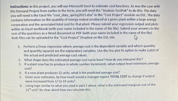
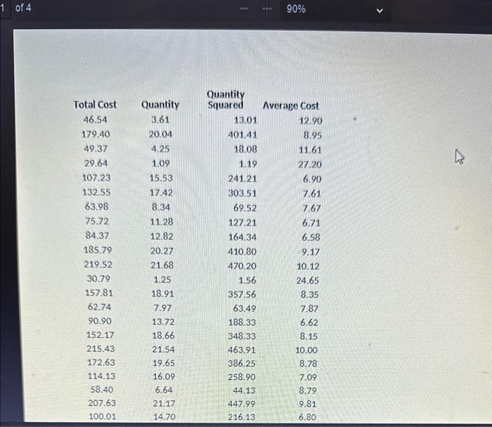
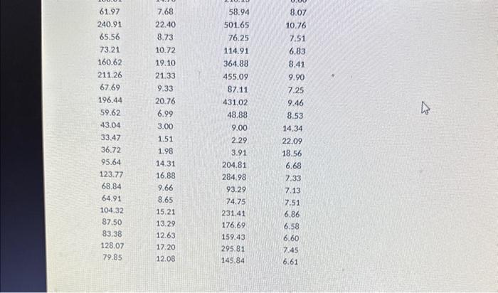
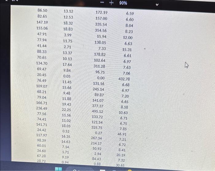
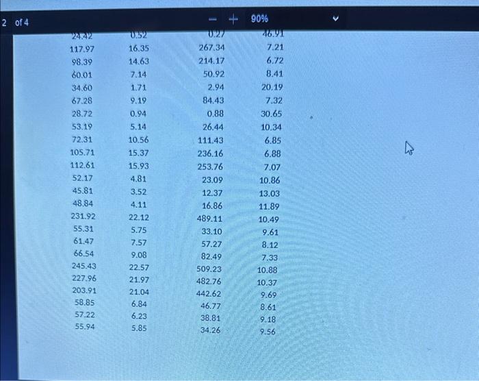
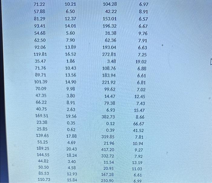
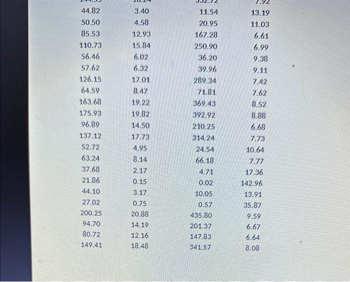
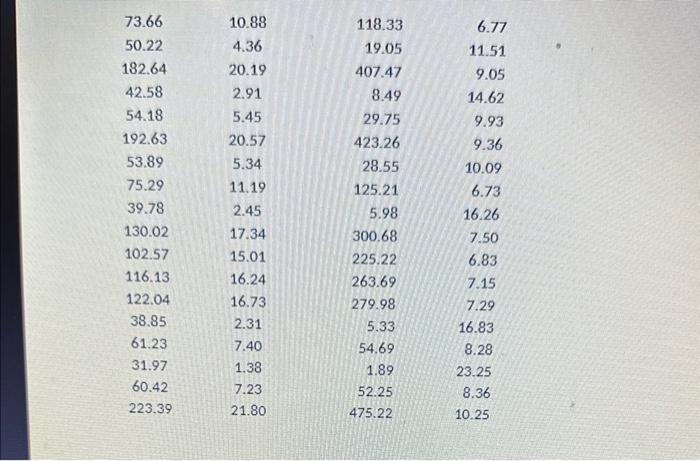
Instructions: In this project, you will use Microsoft Excel to estimate cost functions. As was the case with the Demand Project from earlier in the term, you will need the "Analysis ToolPak" to do this. The data you will need is the Excel file "cost_data_spring2023 xlsx" in the "Cost Project" module on D2L. The data contains information on the quantity of energy output produced at a given plant within a large energy corporation and the associated total cost for that plant. Please submit your regression output and plots within an Excel workbook (with your name included in the name of the file). Submit your answers to the rest of the questions as a Word document or PDF (with your name included in the name of the file). Both files can be uploaded to the "Cost Project" Dropbox on the D2L site. 1. Perform a linear regression where average cost is the dependent variable and where quantity and quantity squared are the explanatory variables. Use the line plot fit option to make a plot of the actual and predicted average cost values. 2. What shape does the estimated average cost curve have? How do you interpret this? 3. If a plant now has to produce in whole number increments, what output level minimizes average cost? 4. If a new plant produces 22 units, what is the predicted average cost? 5. Given your estimates, by how much would a manager expect TOTAL COST to change if output were increased from 17 to 19 units? 6. Using logic similar to what you used in part 5 above, what is the estimated marginal cost of the 21 unit? Be clear about how you calculate this. 1 of 4 \begin{tabular}{ccrrr} Total Cost & Quantity & QuantitySquared & Average Cost \\ 46.54 & 3.61 & 13.01 & 12.90 \\ 179.40 & 20.04 & 401.41 & 8.95 \\ 49.37 & 4.25 & 18.08 & 11.61 \\ 29.64 & 1.09 & 1.19 & 27.20 \\ 107.23 & 15.53 & 241.21 & 6.90 \\ 132.55 & 17.42 & 303.51 & 7.61 \\ 63.98 & 8.34 & 69.52 & 7.67 \\ 75.72 & 11.28 & 127.21 & 6.71 \\ 84.37 & 12.82 & 164.34 & 6.58 \\ 185.79 & 20.27 & 410.80 & 9.17 \\ 219.52 & 21.68 & 470.20 & 10.12 \\ 30.79 & 1.25 & 1.56 & 24.65 \\ 157.81 & 18.91 & 357.56 & 8.35 \\ 62.74 & 7.97 & 63.49 & 7.87 \\ 90.90 & 13.72 & 188.33 & 6.62 \\ 152.17 & 18.66 & 348.33 & 8.15 \\ \hline 215.43 & 21.54 & 463.91 & 10.00 \\ 172.63 & 19.65 & 386.25 & 8.78 \\ 114.13 & 16.09 & 258.90 & 7.09 \\ 58.40 & 6.64 & 44.13 & 8.79 \\ \hline 207.63 & 21.17 & 447.99 & 9.81 \\ 100.01 & 14.70 & 216.13 & 6.80 \\ \hline \end{tabular} \begin{tabular}{ccrr} \hline 61.97 & 7.68 & 58.94 & 8.07 \\ 240.91 & 22.40 & 501.65 & 10.76 \\ 65.56 & 8.73 & 76.25 & 7.51 \\ 73.21 & 10.72 & 114.91 & 6.83 \\ 160.62 & 19.10 & 364.88 & 8.41 \\ 211.26 & 21.33 & 455.09 & 9.90 \\ 67.69 & 9.33 & 87.11 & 7.25 \\ 196.44 & 20.76 & 431.02 & 9.46 \\ 59.62 & 6.99 & 48.88 & 8.53 \\ 43.04 & 3.00 & 9.00 & 14.34 \\ 33.47 & 1.51 & 2.29 & 22.09 \\ 36.72 & 1.98 & 3.91 & 18.56 \\ 95.64 & 14.31 & 204.81 & 6.68 \\ 123.77 & 16.88 & 284.98 & 7.33 \\ 68.84 & 9.66 & 93.29 & 7.13 \\ 64.91 & 8.65 & 74.75 & 7.51 \\ 104.32 & 15.21 & 231.41 & 6.86 \\ 87.50 & 13.29 & 176.69 & 6.58 \\ 83.38 & 12.63 & 159.43 & 6.60 \\ 128.07 & 17.20 & 295.81 & 7.45 \\ 79.85 & 12.08 & 145.84 & 6.61 \end{tabular} \begin{tabular}{|rrrr} \hline 86.50 & 13.12 & 172.19 & 6.59 \\ 82.65 & 12.53 & 157.00 & 6.60 \\ 147.19 & 18.32 & 335.54 & 8.04 \\ 155.06 & 18.83 & 354.56 & 8.23 \\ 47.91 & 3.99 & 15.94 & 12.00 \\ 77.94 & 11.75 & 138.05 & 6.63 \\ 41.44 & 2.71 & 7.33 & 15.31 \\ 88.33 & 13.37 & 178.82 & 6.61 \\ 70.65 & 10.13 & 102.64 & 6.97 \\ 134.70 & 17.64 & 311.28 & 7.63 \\ 69.47 & 9.84 & 96.75 & 7.06 \\ 20.45 & 0.05 & 0.00 & 432.78 \\ 76.49 & 11.45 & 131.16 & 6.68 \\ 109.07 & 15.66 & 245.14 & 6.97 \\ 68.21 & 9.48 & 89.87 & 7.20 \\ 79.04 & 11.88 & 141.07 & 6.65 \\ 166.71 & 19.43 & 377.37 & 8.58 \\ \hline 236.49 & 22.25 & 495.12 & 10.63 \\ \hline 77.56 & 11.56 & 133.72 & 6.71 \\ \hline 74.41 & 11.02 & 121.54 & 6.75 \\ 141.71 & 18.05 & 325.75 & 7.85 \\ \hline 24.42 & 0.52 & 0.27 & 46.91 \\ 117.97 & 16.35 & 267.34 & 7.21 \\ 98.39 & 14.63 & 214.17 & 6.72 \\ 60.01 & 7.14 & 50.92 & 8.41 \\ \hline 34.60 & 1.71 & 8.94 & 20.19 \\ 67.28 & 9.19 & 0.83 & 7.32 \\ \hline 28.72 & 0.94 & 30.65 \\ \hline & & & \\ \hline \end{tabular} 2 of 4 \begin{tabular}{rcrr} 71.22 & 10.21 & 104.28 & 6.97 \\ 57.88 & 6.50 & 42.22 & 8.91 \\ 81.29 & 12.37 & 153.01 & 6.57 \\ 93.41 & 14.01 & 196.32 & 6.67 \\ 54.68 & 5.60 & 31.38 & 9.76 \\ 62.50 & 7.90 & 62.36 & 7.91 \\ 92.06 & 13.89 & 193.04 & 6.63 \\ 119.81 & 16.52 & 272.81 & 7.25 \\ 35.47 & 1.86 & 3.48 & 19.02 \\ 71.76 & 10.43 & 108.76 & 6.88 \\ 89.71 & 13.56 & 183.94 & 6.61 \\ 101.39 & 14.90 & 221.92 & 6.81 \\ 70.09 & 9.98 & 99.62 & 7.02 \\ 47.35 & 3.80 & 14.47 & 12.45 \\ 66.22 & 8.91 & 79.38 & 7.43 \\ 40.75 & 2.63 & 6.93 & 15.47 \\ 169.51 & 19.56 & 382.73 & 8.66 \\ \hline 23.38 & 0.35 & 0.12 & 66.67 \\ \hline 25.85 & 0.62 & 0.39 & 41.52 \\ 139.65 & 17.88 & 319.85 & 7.81 \\ \hline 51.25 & 4.69 & 21.96 & 10.94 \\ 189.25 & 20.43 & 417.20 & 9.27 \\ \hline 144.55 & 18.24 & 332.72 & 7.92 \\ \hline 44.82 & 3.40 & 11.54 & 13.19 \\ \hline 50.50 & 4.58 & 20.95 & 11.03 \\ 85.53 & 12.93 & 167.28 & 6.61 \\ 110.73 & 15.84 & 250.90 & 6.99 \\ \hline \end{tabular} \begin{tabular}{ccrr} 44.82 & 3.40 & 11.54 & 13.19 \\ 50.50 & 4.58 & 20.95 & 11.03 \\ 85.53 & 12.93 & 167.28 & 6.61 \\ 110.73 & 15.84 & 250.90 & 6.99 \\ 56.46 & 6.02 & 36.20 & 9.38 \\ 57.62 & 6.32 & 39.96 & 9.11 \\ 126.15 & 17.01 & 289.34 & 7.42 \\ 64.59 & 8.47 & 71.81 & 7.62 \\ 163.68 & 19.22 & 369.43 & 8.52 \\ 175.93 & 19.82 & 392.92 & 8.88 \\ 96.89 & 14.50 & 210.25 & 6.68 \\ 137.12 & 17.73 & 314.24 & 7.73 \\ 52.72 & 4.95 & 24.54 & 10.64 \\ 63.24 & 8.14 & 66.18 & 7.77 \\ 37.68 & 2.17 & 4.71 & 17.36 \\ 21.86 & 0.15 & 0.02 & 142.96 \\ 44.10 & 3.17 & 10.05 & 13.91 \\ 27.02 & 0.75 & 0.57 & 35.87 \\ 200.25 & 20.88 & 435.80 & 9.59 \\ 94.70 & 14.19 & 201.37 & 6.67 \\ \hline 80.72 & 12.16 & 147.83 & 6.64 \\ 149.41 & 18.48 & 341.57 & 8.08 \\ \hline \end{tabular} 73.6650.22182.6442.5854.18192.6353.8975.2939.78130.02102.57116.13122.0438.8561.2331.9760.42223.3910.884.3620.192.915.4520.575.3411.192.4517.3415.0116.2416.732.317.401.387.2321.80118.3319.05407.478.4929.75423.2628.55125.215.98300.68225.22263.69279.985.3354.691.8952.25475.226.7711.519.0514.629.939.3610.096.7316.267.506.837.157.2916.838.2823.258.3610.25 Instructions: In this project, you will use Microsoft Excel to estimate cost functions. As was the case with the Demand Project from earlier in the term, you will need the "Analysis ToolPak" to do this. The data you will need is the Excel file "cost_data_spring2023 xlsx" in the "Cost Project" module on D2L. The data contains information on the quantity of energy output produced at a given plant within a large energy corporation and the associated total cost for that plant. Please submit your regression output and plots within an Excel workbook (with your name included in the name of the file). Submit your answers to the rest of the questions as a Word document or PDF (with your name included in the name of the file). Both files can be uploaded to the "Cost Project" Dropbox on the D2L site. 1. Perform a linear regression where average cost is the dependent variable and where quantity and quantity squared are the explanatory variables. Use the line plot fit option to make a plot of the actual and predicted average cost values. 2. What shape does the estimated average cost curve have? How do you interpret this? 3. If a plant now has to produce in whole number increments, what output level minimizes average cost? 4. If a new plant produces 22 units, what is the predicted average cost? 5. Given your estimates, by how much would a manager expect TOTAL COST to change if output were increased from 17 to 19 units? 6. Using logic similar to what you used in part 5 above, what is the estimated marginal cost of the 21 unit? Be clear about how you calculate this. 1 of 4 \begin{tabular}{ccrrr} Total Cost & Quantity & QuantitySquared & Average Cost \\ 46.54 & 3.61 & 13.01 & 12.90 \\ 179.40 & 20.04 & 401.41 & 8.95 \\ 49.37 & 4.25 & 18.08 & 11.61 \\ 29.64 & 1.09 & 1.19 & 27.20 \\ 107.23 & 15.53 & 241.21 & 6.90 \\ 132.55 & 17.42 & 303.51 & 7.61 \\ 63.98 & 8.34 & 69.52 & 7.67 \\ 75.72 & 11.28 & 127.21 & 6.71 \\ 84.37 & 12.82 & 164.34 & 6.58 \\ 185.79 & 20.27 & 410.80 & 9.17 \\ 219.52 & 21.68 & 470.20 & 10.12 \\ 30.79 & 1.25 & 1.56 & 24.65 \\ 157.81 & 18.91 & 357.56 & 8.35 \\ 62.74 & 7.97 & 63.49 & 7.87 \\ 90.90 & 13.72 & 188.33 & 6.62 \\ 152.17 & 18.66 & 348.33 & 8.15 \\ \hline 215.43 & 21.54 & 463.91 & 10.00 \\ 172.63 & 19.65 & 386.25 & 8.78 \\ 114.13 & 16.09 & 258.90 & 7.09 \\ 58.40 & 6.64 & 44.13 & 8.79 \\ \hline 207.63 & 21.17 & 447.99 & 9.81 \\ 100.01 & 14.70 & 216.13 & 6.80 \\ \hline \end{tabular} \begin{tabular}{ccrr} \hline 61.97 & 7.68 & 58.94 & 8.07 \\ 240.91 & 22.40 & 501.65 & 10.76 \\ 65.56 & 8.73 & 76.25 & 7.51 \\ 73.21 & 10.72 & 114.91 & 6.83 \\ 160.62 & 19.10 & 364.88 & 8.41 \\ 211.26 & 21.33 & 455.09 & 9.90 \\ 67.69 & 9.33 & 87.11 & 7.25 \\ 196.44 & 20.76 & 431.02 & 9.46 \\ 59.62 & 6.99 & 48.88 & 8.53 \\ 43.04 & 3.00 & 9.00 & 14.34 \\ 33.47 & 1.51 & 2.29 & 22.09 \\ 36.72 & 1.98 & 3.91 & 18.56 \\ 95.64 & 14.31 & 204.81 & 6.68 \\ 123.77 & 16.88 & 284.98 & 7.33 \\ 68.84 & 9.66 & 93.29 & 7.13 \\ 64.91 & 8.65 & 74.75 & 7.51 \\ 104.32 & 15.21 & 231.41 & 6.86 \\ 87.50 & 13.29 & 176.69 & 6.58 \\ 83.38 & 12.63 & 159.43 & 6.60 \\ 128.07 & 17.20 & 295.81 & 7.45 \\ 79.85 & 12.08 & 145.84 & 6.61 \end{tabular} \begin{tabular}{|rrrr} \hline 86.50 & 13.12 & 172.19 & 6.59 \\ 82.65 & 12.53 & 157.00 & 6.60 \\ 147.19 & 18.32 & 335.54 & 8.04 \\ 155.06 & 18.83 & 354.56 & 8.23 \\ 47.91 & 3.99 & 15.94 & 12.00 \\ 77.94 & 11.75 & 138.05 & 6.63 \\ 41.44 & 2.71 & 7.33 & 15.31 \\ 88.33 & 13.37 & 178.82 & 6.61 \\ 70.65 & 10.13 & 102.64 & 6.97 \\ 134.70 & 17.64 & 311.28 & 7.63 \\ 69.47 & 9.84 & 96.75 & 7.06 \\ 20.45 & 0.05 & 0.00 & 432.78 \\ 76.49 & 11.45 & 131.16 & 6.68 \\ 109.07 & 15.66 & 245.14 & 6.97 \\ 68.21 & 9.48 & 89.87 & 7.20 \\ 79.04 & 11.88 & 141.07 & 6.65 \\ 166.71 & 19.43 & 377.37 & 8.58 \\ \hline 236.49 & 22.25 & 495.12 & 10.63 \\ \hline 77.56 & 11.56 & 133.72 & 6.71 \\ \hline 74.41 & 11.02 & 121.54 & 6.75 \\ 141.71 & 18.05 & 325.75 & 7.85 \\ \hline 24.42 & 0.52 & 0.27 & 46.91 \\ 117.97 & 16.35 & 267.34 & 7.21 \\ 98.39 & 14.63 & 214.17 & 6.72 \\ 60.01 & 7.14 & 50.92 & 8.41 \\ \hline 34.60 & 1.71 & 8.94 & 20.19 \\ 67.28 & 9.19 & 0.83 & 7.32 \\ \hline 28.72 & 0.94 & 30.65 \\ \hline & & & \\ \hline \end{tabular} 2 of 4 \begin{tabular}{rcrr} 71.22 & 10.21 & 104.28 & 6.97 \\ 57.88 & 6.50 & 42.22 & 8.91 \\ 81.29 & 12.37 & 153.01 & 6.57 \\ 93.41 & 14.01 & 196.32 & 6.67 \\ 54.68 & 5.60 & 31.38 & 9.76 \\ 62.50 & 7.90 & 62.36 & 7.91 \\ 92.06 & 13.89 & 193.04 & 6.63 \\ 119.81 & 16.52 & 272.81 & 7.25 \\ 35.47 & 1.86 & 3.48 & 19.02 \\ 71.76 & 10.43 & 108.76 & 6.88 \\ 89.71 & 13.56 & 183.94 & 6.61 \\ 101.39 & 14.90 & 221.92 & 6.81 \\ 70.09 & 9.98 & 99.62 & 7.02 \\ 47.35 & 3.80 & 14.47 & 12.45 \\ 66.22 & 8.91 & 79.38 & 7.43 \\ 40.75 & 2.63 & 6.93 & 15.47 \\ 169.51 & 19.56 & 382.73 & 8.66 \\ \hline 23.38 & 0.35 & 0.12 & 66.67 \\ \hline 25.85 & 0.62 & 0.39 & 41.52 \\ 139.65 & 17.88 & 319.85 & 7.81 \\ \hline 51.25 & 4.69 & 21.96 & 10.94 \\ 189.25 & 20.43 & 417.20 & 9.27 \\ \hline 144.55 & 18.24 & 332.72 & 7.92 \\ \hline 44.82 & 3.40 & 11.54 & 13.19 \\ \hline 50.50 & 4.58 & 20.95 & 11.03 \\ 85.53 & 12.93 & 167.28 & 6.61 \\ 110.73 & 15.84 & 250.90 & 6.99 \\ \hline \end{tabular} \begin{tabular}{ccrr} 44.82 & 3.40 & 11.54 & 13.19 \\ 50.50 & 4.58 & 20.95 & 11.03 \\ 85.53 & 12.93 & 167.28 & 6.61 \\ 110.73 & 15.84 & 250.90 & 6.99 \\ 56.46 & 6.02 & 36.20 & 9.38 \\ 57.62 & 6.32 & 39.96 & 9.11 \\ 126.15 & 17.01 & 289.34 & 7.42 \\ 64.59 & 8.47 & 71.81 & 7.62 \\ 163.68 & 19.22 & 369.43 & 8.52 \\ 175.93 & 19.82 & 392.92 & 8.88 \\ 96.89 & 14.50 & 210.25 & 6.68 \\ 137.12 & 17.73 & 314.24 & 7.73 \\ 52.72 & 4.95 & 24.54 & 10.64 \\ 63.24 & 8.14 & 66.18 & 7.77 \\ 37.68 & 2.17 & 4.71 & 17.36 \\ 21.86 & 0.15 & 0.02 & 142.96 \\ 44.10 & 3.17 & 10.05 & 13.91 \\ 27.02 & 0.75 & 0.57 & 35.87 \\ 200.25 & 20.88 & 435.80 & 9.59 \\ 94.70 & 14.19 & 201.37 & 6.67 \\ \hline 80.72 & 12.16 & 147.83 & 6.64 \\ 149.41 & 18.48 & 341.57 & 8.08 \\ \hline \end{tabular} 73.6650.22182.6442.5854.18192.6353.8975.2939.78130.02102.57116.13122.0438.8561.2331.9760.42223.3910.884.3620.192.915.4520.575.3411.192.4517.3415.0116.2416.732.317.401.387.2321.80118.3319.05407.478.4929.75423.2628.55125.215.98300.68225.22263.69279.985.3354.691.8952.25475.226.7711.519.0514.629.939.3610.096.7316.267.506.837.157.2916.838.2823.258.3610.25