its Assignment topic

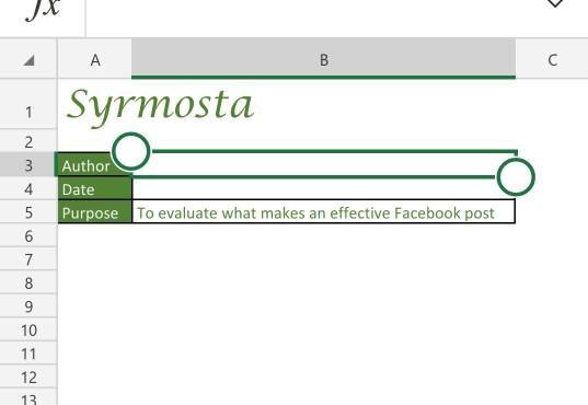
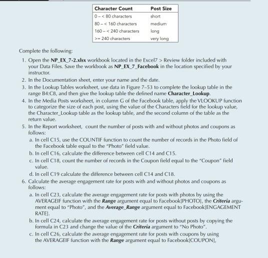
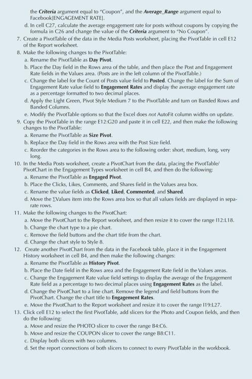
4 A B 1 Syrmosta N 4 5 2 3 4 5 6 Author Date Purpose To evaluate what makes an effective Facebook post 9 7 8 9 10 11 12 13 Character Count 0 - 240 characters Post Size short medium long very long Complete the following: 1. Open the NP_EX_7-2.xlsx workbook located in the Excel7 > Review folder included with your Data Files. Save the workbook as NP EX 7 Facebook in the location specified by your instructor 2. In the Documentation sheet, enter your name and the date. 3. In the Lookup Tables worksheet, use data in Figure 7-53 to complete the lookup table in the range B4:C8, and then give the lookup table the defined name Character_Lookup. 4. In the Media Posts worksheet, in column G of the Facebook table, apply the VLOOKUP function to categorize the size of each post, using the value of the Characters field for the lookup value, the Character Lookup table as the lookup table, and the second column of the table as the return value 5. In the Report worksheet, count the number of posts with and without photos and coupons as follows: a. In cell C15, use the COUNTIF function to count the number of records in the Photo field of the Facebook table equal to the Photo" field value. b. In cell C16, calculate the difference between cell C14 and C15, c. In cell C18, count the number of records in the Coupon field equal to the "Coupon" field value. d. In cell C19 calculate the difference between cell C14 and C18. 6. Calculate the average engagement rate for posts with and without photos and coupons as follows: a. In cell C23, calculate the average engagement rate for posts with photos by using the AVERAGEIF function with the Range argument equal to Facebook PHOTOS, the Criteria argu- ment equal to "Photo", and the Average Range argument equal to Facebook/ENGAGEMENT RATE b. In cell C24, calculate the average engagement rate for posts without posts by copying the formula in C23 and change the value of the Criteria argument to "No Photo". c. In cell C26, calculate the average engagement rate for posts with coupons by using the AVERAGEIF function with the Range argument equal to Facebook[COUPONI, the Criteria argument equal to "Coupon", and the Average_Range argument equal to Facebook ENGAGEMENT RATED d. In cell C27, calculate the average engagement rate for posts without coupons by copying the formula in C26 and change the value of the Criteria argument to "No Coupon 7. Create a Pivot Table of the data in the Media Posts worksheet, placing the Pivot Table in cell E12 of the Report worksheet 8. Make the following changes to the Pivot Table: a. Rename the Pivot Table as Day Pivot. b. Place the Day field in the Rows area of the table, and then place the Post and Engagement Rate fields in the Values area. (Posts are in the left column of the Pivot Table.) c. Change the label for the Count of Posts value field to Posted. Change the label for the Sum of Engagement Rate value field to Engagement Rates and display the average engagement rate as a percentage formatted to two decimal places. d. Apply the Light Green, Pivot Style Medium 7 to the Pivot Table and tum on Banded Rows and Banded Columns e. Modify the Pivot Table options so that the Excel does not AutoFit column widths on update. 9. Copy the Pivot Table in the range E12:20 and paste it in cell E22, and then make the following changes to the Pivot Table: a. Rename the Pivot Table as Size Pivot. b. Replace the Day field in the Rows area with the Post Size field c. Reorder the categories in the Rows area to the following order:short, medium, long, very long 10. In the Media Posts worksheet, create a PivotChart from the data, placing the Pivot Table/ PivotChart in the Engagement Types worksheet in cell B4, and then do the following: a. Rename the Pivot Table as Engaged Pivot. b. Place the Clicks, Like, Comments and Shares field in the Values area box. c. Rename the value fields as Clicked Liked, Commented, and Shared, d. Move the values item into the Rows area box so that all values fields are displayed in sepa- rate rows. 11. Make the following changes to the PivotChart: a. Move the PivotChart to the Report worksheet, and then resize it to cover the range 112:118. b. Change the chart type to a ple chart c. Remove the field buttons and the chart title from the chart. d. Change the chart style to Style 8. 12. Create another PivotChart from the data in the Facebook table, place it in the Engagement History worksheet in cell B4, and then make the following changes a. Rename the Pivot Table as History Pivot. b. Place the Date field in the Rows area and the Engagement Rate field in the values areas. c. Change the Engagement Rate value field settings to display the average of the Engagement Rate field as a percentage to two decimal places using Engagement Rates as the label d. Change the PivotChart to a line chart. Remove the legend and field buttons from the PivotChart Change the chart title to Engagement Rates e. Move the PivotChart to the Report worksheet and resize it to cover the range 119:127. 13. Click cell E12 to select the first Pivot Table, add slicers for the photo and Coupon fields, and then do the following a. Move and resize the PHOTO slicer to cover the range B4:06. b. Move and resize the COUPON slicer to cover the range B8:C11. c. Display both slicers with two columns. d. Set the report connections of both slicers to connect to every Pivot Table in the workbook