k$.$ Modify cell $K8$ to show two places after the decimal.

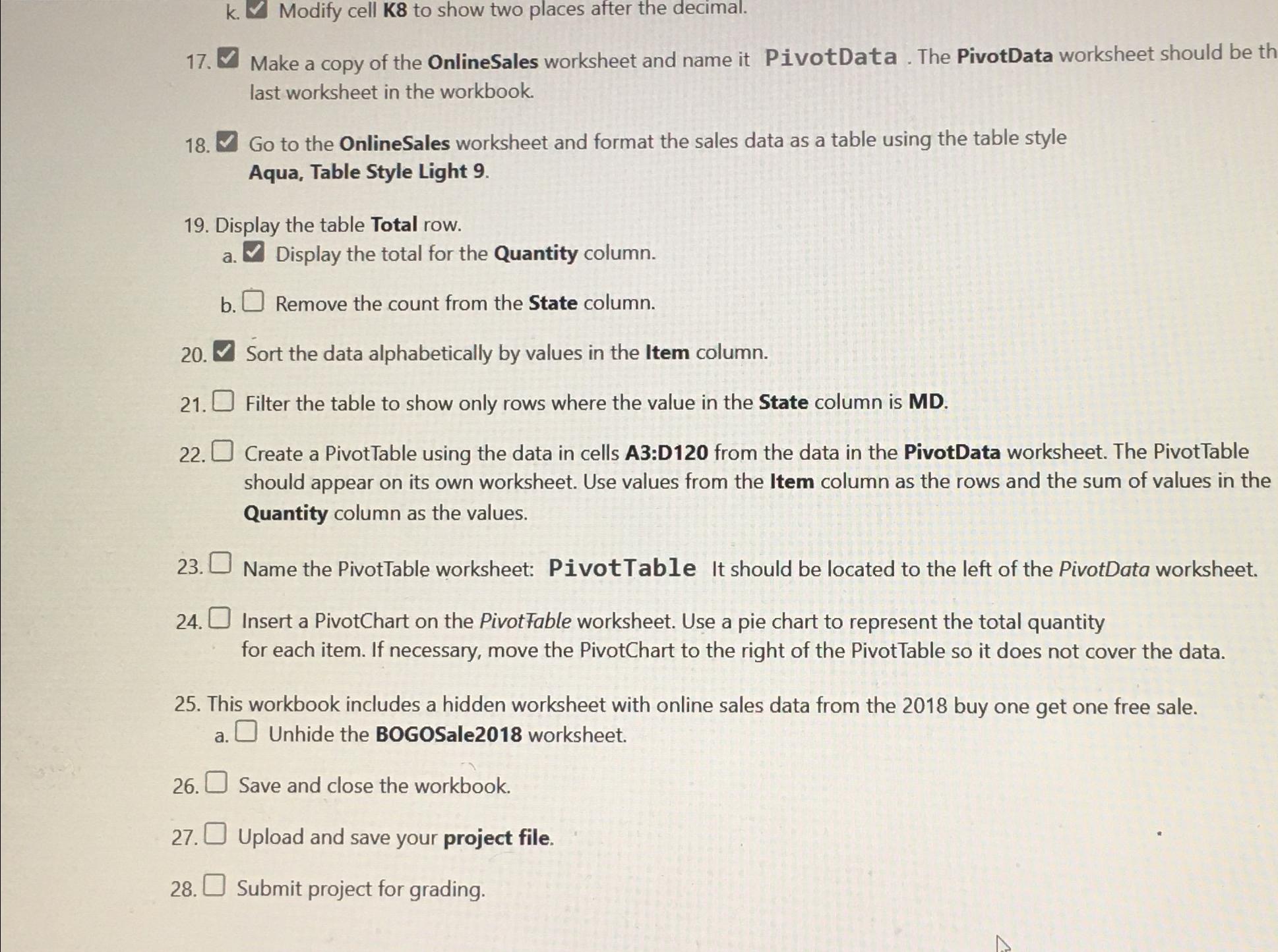
$17.$ Make a copy of the OnlineSales worksheet and name it PivotData $.$ The PivotData worksheet should be th last worksheet in the workbook.

$18.$ Go to the OnlineSales worksheet and format the sales data as a table using the table style Aqua, Table Style Light $9.$

$19.$ Display the table Total row.

a$.$ Display the total for the Quantity column.

b$.$ Remove the count from the State column.

$20.$ Sort the data alphabetically by values in the Item column.

$21.$ Filter the table to show only rows where the value in the State column is MD$.$

$22.$ Create a PivotTable using the data in cells A$3$:D$120$ from the data in the PivotData worksheet. The PivotTable should appear on its own worksheet. Use values from the Item column as the rows and the sum of values in the Quantity column as the values.

$23.$ Name the PivotTable worksheet: PivotTable It should be located to the left of the PivotData worksheet.

$24.$ Insert a PivotChart on the PivotFable worksheet. Use a pie chart to represent the total quantity for each item. If necessary, move the PivotChart to the right of the PivotTable so it does not cover the data.

$25.$ This workbook includes a hidden worksheet with online sales data from the $2018$ buy one get one free sale.

a$.$ Unhide the BOGOSale$2018$ worksheet.

$26.$ Save and close the workbook.

$27.$ Upload and save your project file.

$28.$ Submit project for grading.