(matlab code only) (matlab code only) (matlab code only) (matlab code only) (matlab code only) (matlab code only) (matlab code only) (matlab code only) (matlab code only) (matlab code only) (matlab code only)

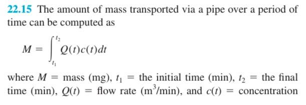
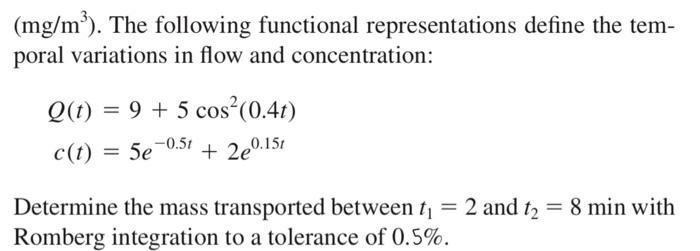
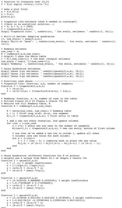
Repeat Problem 22.15: Using 5-point and 6-point Gauss quadrature. Compare to your answer from the previous problem, and also compare to the result using the built-in quad function. 22.15 The amount of mass transported via a pipe over a period of time can be computed as M = Q(1)c(1)dt where M = mass (mg), t the initial time (min), 12 the final time (min), Q(t) = flow rate (m/min), and c(t) = concentration (mg/m). The following functional representations define the tem- poral variations in flow and concentration: Q(t) c(t) = 5e-0.51 = 9 + 5 cos?(0.4t) 5e -0.51 + 2e0.151 Determine the mass transported between t1 = 2 and t2 = 8 min with Romberg integration to a tolerance of 0.5%. function to integrate over 10,2) f - x) exp(x)..sin(x)./(1+x.-2); make a plot first X-010.01:21 y = f(x): plot(x,y); trapezoid rule estimate (what h needed to converge?) (there is no analytical solution...) - - 0; b - 21 - 2000; I trapezoide, a,b,n) di spettrapezoid rule: . num2strin). * Exnevals, estinate: nun2str I. 1611) Built-in Matlabi Adaptive quadrature di spi! Built-in "quad: hun2strinum_evals) .txe ovals, estimatet numstre. Romberg estimate num_rows - 4: R - romberg, a,b,numrows) dispiR) show the whole table 1 - Rinun_row+1); the best Integral estimate num_evals - sum 2. 1. num_rows+1)): dispe Romberg: , num stefnun evala), Exnevals, estimate: numat(I, 16) Gauss Quadraturo estimates dispil'Gauss 2-pt estimate: 'numst gauss(f, a,b), 16)); displGauss 3-pt estimate: num2ste gauss 3.a,b), 16)); displ'Gauss 4-pt estimates num2 strgauss(f, a,b), 1651) Punctions used above: Trapezoid rule: function, a,b. number of segmonts function I - trapezoidif, a,b,n) h = (b-a) I - (h/2)(a) + 2 sunt(athihibh )) + f(b)); end Romberg: function, a, b, number of rows in the table Follows Figure 22.4 of Chapra 4 Canale 7th Ed. Returns the full Romberg tablo, R function R - ronberg(a, b, nam rows) Rzorosinun roVS, nun_rown) Romberg table n-1: first step size: (b-a), one segment (1.1) - trapezoidif.a,b,n); first entry in table add a new row every iteration, and update columns for iter - linum row n = 12; every new row uses 2x the number of segments R(Iter+1.1) - trapezoid!,,b.); new row entry, bottom of first column now that we've added a new row in column 1, update all other columns (one new value for each column) fork - 2. iter 1 1 = 2 + iter - K: Indexing back to place the new value ROD,K) - (4 (k-1). R(+1, k-1) - REJ.K-1))/ (41k-1) - 1) end end end Gauss Quadrature (different functions for of points) weights and values from Table 22.1 of Chapra & Canale 7th function 1 - gauss 2(f.a,b) c=11111 weight coefficients * - !-1/sqrt(3) 1/sqrt{3)); y = (a+b)/2 + (b-a)/2 x; I - (-a)/2 .se. ()) end function I - 483, a.b) 10.5558$56.6, E88 8 889 5.68SSSS6): 1 weight coefficients y - (a+b)/2 + (b-a)/2 x; I = (-a)/2 sumie.173 end function I - gauss(f, a,b) e-10.3478548 0.6521452 0.6521452 0.3478548); weight coefficients * - 1-0.861136312 -0.339981044 0.399981044 0.8611363121 y - (a+b)/2 + (b-a)/2 x 1 = (-a)/2 . sume.f))