(matlab code only) (matlab code only) (matlab code only) (matlab code only) (matlab code only) (matlab code only) (matlab code only) (matlab code only) (matlab code only) (matlab code only) (matlab code only)

this is the teachers question

heres the problem hes refering to

heres the sample code that i need to change/ use

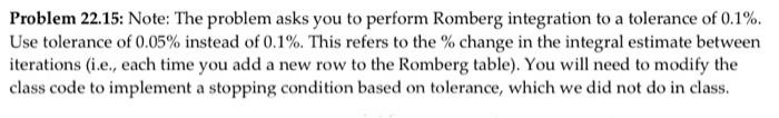
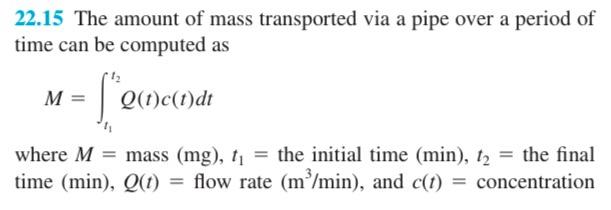
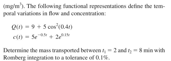
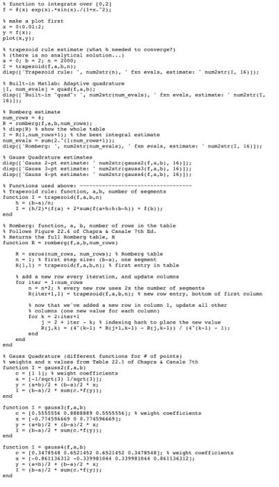
Problem 22.15: Note: The problem asks you to perform Romberg integration to a tolerance of 0.1%. Use tolerance of 0.05% instead of 0.1%. This refers to the % change in the integral estimate between iterations (ie., each time you add a new row to the Romberg table). You will need to modify the class code to implement a stopping condition based on tolerance, which we did not do in class. 22.15 The amount of mass transported via a pipe over a period of time can be computed as M = Q(1)c(1)dt where M = mass (mg), t the initial time (min), 12 the final time (min), Q(t) = flow rate (m/min), and c(t) = concentration (mg/m). The following functional representations define the tem- poral variations in flow and concentration: Q(t) = 9 + 5 cos?(0.41) c(t) = 5e +0.51 + 2e0.151 Determine the mass transported between t1 = 2 and t2 = 8 min with Romberg integration to a tolerance of 0.1%. function to integrate over 10,21 =**) exp(x).sin(x)/(1+x. 2): make a plot first X-010.0112 y = f(x): plot*,): trapezoid rule estimate what he needed to converge?) (there is no analytical solution...) a. 0; b. 2; n2000; I trapezoidit,,b.n) displ Traperoid rulei, numstrin). Exnevats, estimate: Str. 1671) Built-in Matlab: Adaptive quadrature 11, nun evals! - quadct,a,b); disp Built-in "quad.numstrinun_evals), fan evals, estimate: numatri, 16)) Romberg estimate num_rows - Rronbergit.a, b, numrove) disp() show the whole table 1 . RC1, num_rowa +1); the best integral estimate despit "Romberg, numetrinun_evais, Exnevals, estimate numer 11, 36) Gauss Quadrature estimates displt Gauss 2-pt estimate namastrgaus 82(1,2,b), 16)) displl Gauss 3-pt estimate: nustegauss 3.a,b). 1671) dispil Gauss 4-pt estimate: numst aussit.a,b). 16) 1); Punetions used above: Trapezoid rule: function, a,b, number of segments function I - trapezoid(f.a,b,n) h = (-a): 1 = (1/2)*(a) + 2*suntf(a+hahb-hi) ton end Rombergi function, a, b, number of rows in the table 9 Follows Figure 22.4 of Chapra Canale 7th Ed. Returns the full Romberg table. R function - Tombergi,,b,nun rows - zeros inun_rowa, nun_rows): Ronberg table n. 1; first step siset (-a), one segment R41,1) - trapezoid(fab.n) first entry in table add a new row every iteration, and update columns for Iter - 1.nun rows - n2: every new row uses 2x the number of segments Reiter+1,1) - trapezoid.&.b.n) new row entry, bottom of first column now that we've added a new row in column 1, update all other columns (one new value for each column) Eork - 2:iter! - 2 + iter -ki indexing hack to place the new value RU,X) - ( 4-1). R(+1,-1) - R.K-1)) / 4 (k-1) - 3) end end end Gauss Quadrature (different functions for of points) weights and x values from Table 22.1 of Chapra Canale 7th function 1- gauss(a,b) c=111) weight coefficients * - -1/aqrt(3) 1/get(3)]: y (a+b)/2 = (-a)/2 X (b-a)/2 aume. (Y) ond function 1 = gauss(1,a,b) c10.5555556 0. SEBEEST 0.5555556); weight coefficients * - 1 -0.774596669 0.72459666911 y - (a+b)/2 + (-a)/2 X I = (b-a)/2 sum(c.ffy) end function Igaun(...) c - 10.3478548 0.6521452 0.6521452 0.3478548); t weight coefficients * - -0.861136312 -0.339981044 0.339981044 0.8611363123 Y - (a+b)/2 (-a)/2 X I= (-a)/2 sume. (y) end