

Question: Microsoft | Excel + Power Query Open the Lab 2 - 2 Slainte Model.xlsx you created in Part 1 . Click the Insert tab on
Microsoft Excel Power Query
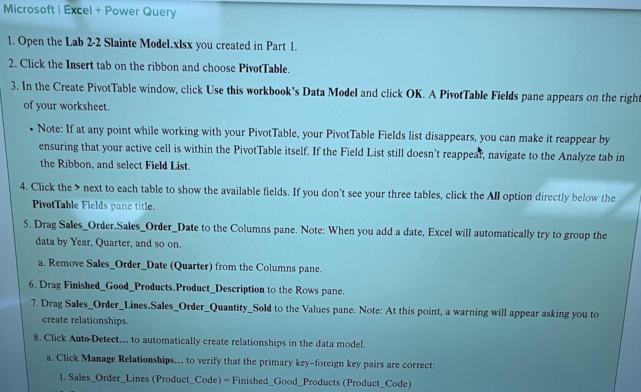
Open the Lab Slainte Model.xlsx you created in Part
Click the Insert tab on the ribbon and choose PivotTable.
In the Create PivotTable window, click Use this workbook's Data Model and click OK A PivotTable Fields pane appears on the right of your worksheet.
Note: If at any point while working with your PivotTable, your PivotTable Fields list disappears, you can make it reappear by ensuring that your active cell is within the PivotTable itself. If the Field List still doesn't reappeat, navigate to the Analyze tab in the Ribbon, and select Field List.
Click the next to each table to show the available fields. If you don't see your three tables, click the All option directly below the PivotTable Fields pane title.
Drag SalesOrder.SalesOrderDate to the Columns pane. Note: When you add a date, Excel will automatically try to group the data by Year, Quarter, and so on
a Remove SalesOrderDate Quarter from the Columns pane.
Drag FinishedGoodProducts.ProductDescription to the Rows pane.
Drag SalesOrderLines.SalesOrderQuantitySold to the Values pane. Note: At this point, a warning will appear asking you to create relationships.
Click AutoDetect... to automatically create relationships in the data model.
a Click Manage Relationships... to verify that the primary keyforeign key pairs are correct:
SalesOrderLines ProductCode FinishedGoodProducts ProductCode
Step by Step Solution
There are 3 Steps involved in it
1 Expert Approved Answer
Step: 1 Unlock

Question Has Been Solved by an Expert!
Get step-by-step solutions from verified subject matter experts
Step: 2 Unlock
Step: 3 Unlock