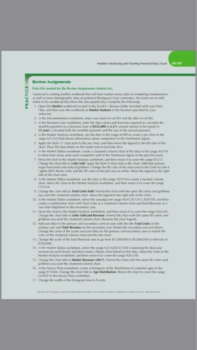
Module 4 Analyaing and Charting Financial DataExc Review Assignments Data File needed for the Review Awignmentsc Market.alex Haywood is ceating another wokbook thut wil huve market survey data on competing mandacturs an well as more demographic dta on potential Backopace Gear customers. He wants you to add charts to his workbook thur show this data graphically,Complese the following U the Market workhook located in the Excel4> Review folder included with your Data Fiks, and then save the workbook as Market Analysis in the location speciied by your 2. in the Documentation worksheet, enter your name in cell 81 and the date in cell 8 I in the Business Loan worksheet, enter the data values and lormulas required to calculate the monthly paymont on alusness loan cf S22s, at 62% annual iterwt to be repaid in 15 years Cakulate bo morehly Payment and ne sue of he annual payment. 4. in the Market Analysis worksheet, une the data in the range A4 89 10 oeate a pie chan in the ange All24 that shows inormation about competitors in the Niowthwest region Applvthe Style 11 chart yle to the pie churt and then move the legendtobelet side od the thart Place the data labeh on the inside end of each pie slice cneate a clusteed colum chat o range AS.FIO to show how many units each competitor sold in the Nonthwest repion in the past five yean 7. Move the chart to the Murket Analysis worlsheet, and then resine it to cover the range E4:113 Chinge the chat tile to Units Sold. Apply the Style 9 chart shyle to the chart. Add both primary eajor horiaontal and vertical gridines. Change the fill color ol the chart area to the Gold Accet 4 upherr ac % derne color and the ill color of the plot area to whte Move the legend to the right & in the Market Tables worksheet, use the data in the range AS F10 to Create a stacked colum churt Move the chart to the Markxt Analysis worksheet, and then resine ito cover the range 9. Change the chart tife to Total Units Sold Form he chart with the same ill colors and grkdlines you used the clustered column chart Move the legend to the right side oif the chart 10. in the Markst Tables worksheet, select the nonadjacent range ASFSA11FI1,A29-529, and then 11. Move the chart to the Market Analysis worksheet and then esine it to cover the range 126:140 12. Add axis tifes to the primary and secondary vertical aves with the tide Total Units on the combination chart with Total Units as a clslered columm chat and Total Revenue ine chart diaplayed on the secondary ash. Change the chart tife to Units Sold and Revenue. Format the chart with the same Gll colors and gridines you ssed the clustered column chart Remove the chat legend primary axis and Tolal Revenue on the secondary a,Rote the secondary andis test down Change the color ol the cales and asis tales for the primary and seconday ases to manch the polor of the clusteeed column chart and the ine chart 14 . Mahr, Tables worksheet, select te range A2 3 AaF23 F28 cutaining the linal year revenue tor each brand, and then create a Pareto chart based on this data. Move the chart to the range A26 C40 15. Change the chart tite to Market Revenue (2017). Formt the chart with the same 6ill colors and gridines you ssed the cludered colmn chart Inthe Survey Dato worksheet, cmne a hisnyam cd the distributon ol customer age, irs tang, E7ES06. Change the chart btle to Age Distrbution Reuze the chart to cover tte rarige G4 P22 in the Survey Data worlsheet 17. Change the width od the histogram bis to 5 units EX 252 Excel | Module 4 Analyzing and Charting Financial Data 18. In the Market Analysis worksheet, add gradient fill orange data bars to the values in the range B5:B9. Set the maximum value of the data bars to 0.6 19. In the range C5:C9, insert line sparklines based on the data in the range B15:F19 of the Market Tables worksheet to show how the competitors' share of the market has changed over the past five years 20. Save the workbook, and then close it. Module 4 Analyaing and Charting Financial DataExc Review Assignments Data File needed for the Review Awignmentsc Market.alex Haywood is ceating another wokbook thut wil huve market survey data on competing mandacturs an well as more demographic dta on potential Backopace Gear customers. He wants you to add charts to his workbook thur show this data graphically,Complese the following U the Market workhook located in the Excel4> Review folder included with your Data Fiks, and then save the workbook as Market Analysis in the location speciied by your 2. in the Documentation worksheet, enter your name in cell 81 and the date in cell 8 I in the Business Loan worksheet, enter the data values and lormulas required to calculate the monthly paymont on alusness loan cf S22s, at 62% annual iterwt to be repaid in 15 years Cakulate bo morehly Payment and ne sue of he annual payment. 4. in the Market Analysis worksheet, une the data in the range A4 89 10 oeate a pie chan in the ange All24 that shows inormation about competitors in the Niowthwest region Applvthe Style 11 chart yle to the pie churt and then move the legendtobelet side od the thart Place the data labeh on the inside end of each pie slice cneate a clusteed colum chat o range AS.FIO to show how many units each competitor sold in the Nonthwest repion in the past five yean 7. Move the chart to the Murket Analysis worlsheet, and then resine it to cover the range E4:113 Chinge the chat tile to Units Sold. Apply the Style 9 chart shyle to the chart. Add both primary eajor horiaontal and vertical gridines. Change the fill color ol the chart area to the Gold Accet 4 upherr ac % derne color and the ill color of the plot area to whte Move the legend to the right & in the Market Tables worksheet, use the data in the range AS F10 to Create a stacked colum churt Move the chart to the Markxt Analysis worksheet, and then resine ito cover the range 9. Change the chart tife to Total Units Sold Form he chart with the same ill colors and grkdlines you used the clustered column chart Move the legend to the right side oif the chart 10. in the Markst Tables worksheet, select the nonadjacent range ASFSA11FI1,A29-529, and then 11. Move the chart to the Market Analysis worksheet and then esine it to cover the range 126:140 12. Add axis tifes to the primary and secondary vertical aves with the tide Total Units on the combination chart with Total Units as a clslered columm chat and Total Revenue ine chart diaplayed on the secondary ash. Change the chart tife to Units Sold and Revenue. Format the chart with the same Gll colors and gridines you ssed the clustered column chart Remove the chat legend primary axis and Tolal Revenue on the secondary a,Rote the secondary andis test down Change the color ol the cales and asis tales for the primary and seconday ases to manch the polor of the clusteeed column chart and the ine chart 14 . Mahr, Tables worksheet, select te range A2 3 AaF23 F28 cutaining the linal year revenue tor each brand, and then create a Pareto chart based on this data. Move the chart to the range A26 C40 15. Change the chart tite to Market Revenue (2017). Formt the chart with the same 6ill colors and gridines you ssed the cludered colmn chart Inthe Survey Dato worksheet, cmne a hisnyam cd the distributon ol customer age, irs tang, E7ES06. Change the chart btle to Age Distrbution Reuze the chart to cover tte rarige G4 P22 in the Survey Data worlsheet 17. Change the width od the histogram bis to 5 units EX 252 Excel | Module 4 Analyzing and Charting Financial Data 18. In the Market Analysis worksheet, add gradient fill orange data bars to the values in the range B5:B9. Set the maximum value of the data bars to 0.6 19. In the range C5:C9, insert line sparklines based on the data in the range B15:F19 of the Market Tables worksheet to show how the competitors' share of the market has changed over the past five years 20. Save the workbook, and then close it