Need help on the following MathLab

Case studied in Ex 2 were as the following

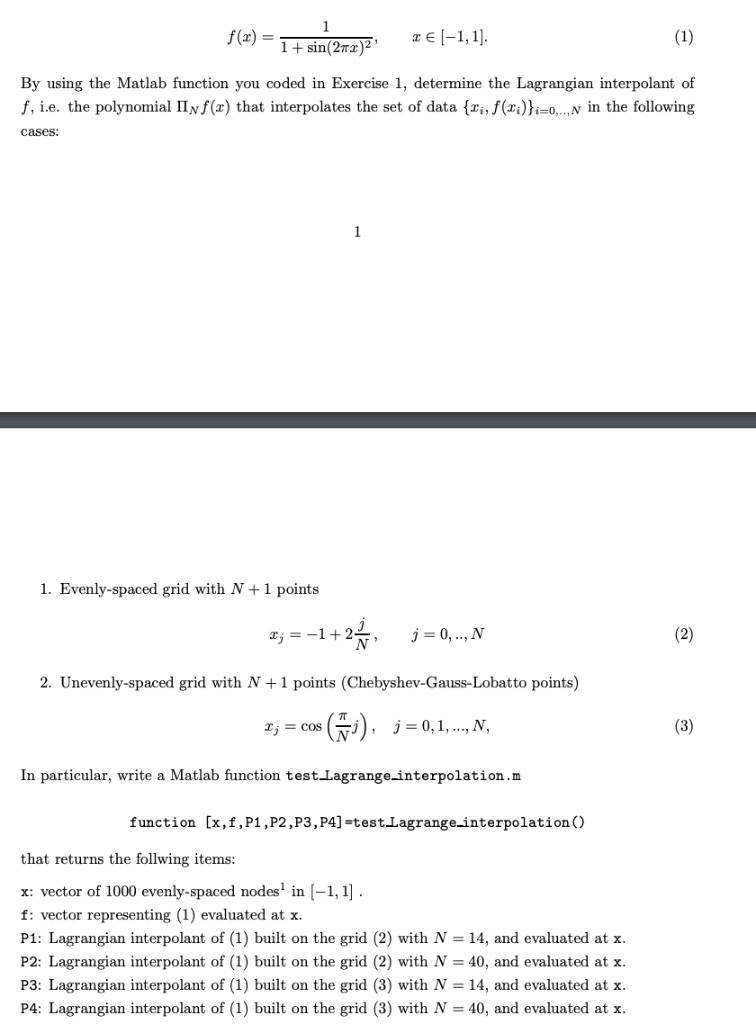
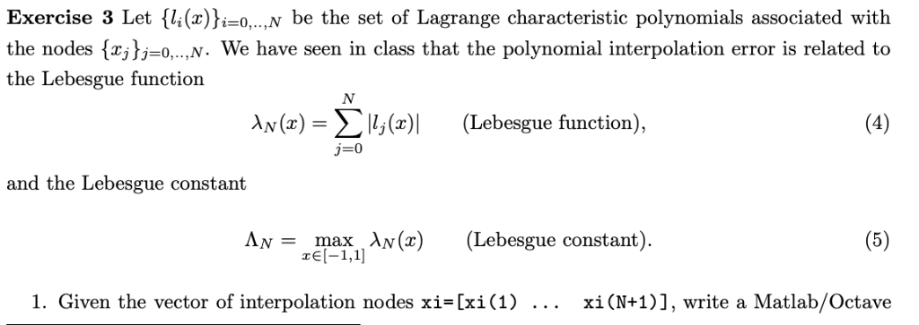
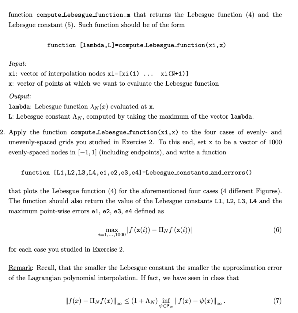
Exercise 3 Let {l(x))i-o,.,N be the set of Lagrange characteristic polynomials associated with the nodes {Fj},=0,..,N. We have seen in class that the polynomial interpolation error is related to the Lebesgue function (x)-,(x)| 3-0 (Lebesgue function), and the Lebesgue constant AN = zmax N(x) (Lebesgue constant). rEl-1,1] 1. Given the vector of interpolation nodes xi-[xi(1) xi(N+1)], write a Matlab/Octave function compute Lebesgue.function.m that returns the Lebesgue function (4) and the Lebesgue constant (5). Such function should be of the form function [lambda,L]-computeLebesgue function(xi,x) Input: xi: vector of interpolation nodes xi-[xi(1) x: vector of points at which we want to evaluate the Lebesgue function Output: lambda: Lebesgue function Xv(x) evaluated at x L: Lebesgue constant Av, computed by taking the maximum of the vector lambda 2. Apply the function computeLebesgue-function(xi,x) to the four cases of evenly- and unevenly-spaced grids you studied in Exercise 2. To this end, set x to be a vector of 1000 evenly-spaced nodes in [-1,1] (including endpoints), and write a function function [LI,L2 , L3,L4, el'e2,e3 , e4]=Lebesgue.constant s-and-errors() that plots the Lebesgue function (4) for the aforementioned four cases (4 different Figures) The function should also return the value of the Lebesgue constants L1, L2, L3, L4 and the maximum point-wise errors e1, e2, e3, e4 defined as i-1,...,1000 for each case you studied in Exercise 2. Remark: Recall, that the smaller the Lebesgue constant the smaller the approximation error of the Lagrangian polynomial interpolation. If fact, we have seen in class that pEPN f(x) +sin(2T)2" By using the Matlab function you coded in Exercise 1, determine the Lagrangian interpolant of f, i.e. the polynomial IIvf(x) that interpolates the set of data [x,, f(xi)H-o,...v in the following cases: I. Evenly-spaced grid with N+1 points 2. Unevenly-spaced grid with N +1 points (Chebyshev-Gauss-Lobatto points) xj =cos (Nj), j=0,1, ,N, In particular, write a Matlab function test Lagrange-interpolation.m function [x,f,P1,P2,P3,P4]-testLagrange-interpolation() that returns the follwing items x: vector of 1000 evenly-spaced nodes in [-1,1] f: vector representing (1) evaluated at x P1: Lagrangian interpolant of (1) built on the grid (2) with N = 14, and evaluated at x P2: Lagrangian interpolant of (1) built on the grid (2) with N = 40, and evaluated at x P3: Lagrangian interpolant of (1) built on the grid (3) with N-14, and evaluated at x P4: Lagrangian interpolant of (1) built on the grid (3) with N 40, and evaluated at x Exercise 3 Let {l(x))i-o,.,N be the set of Lagrange characteristic polynomials associated with the nodes {Fj},=0,..,N. We have seen in class that the polynomial interpolation error is related to the Lebesgue function (x)-,(x)| 3-0 (Lebesgue function), and the Lebesgue constant AN = zmax N(x) (Lebesgue constant). rEl-1,1] 1. Given the vector of interpolation nodes xi-[xi(1) xi(N+1)], write a Matlab/Octave function compute Lebesgue.function.m that returns the Lebesgue function (4) and the Lebesgue constant (5). Such function should be of the form function [lambda,L]-computeLebesgue function(xi,x) Input: xi: vector of interpolation nodes xi-[xi(1) x: vector of points at which we want to evaluate the Lebesgue function Output: lambda: Lebesgue function Xv(x) evaluated at x L: Lebesgue constant Av, computed by taking the maximum of the vector lambda 2. Apply the function computeLebesgue-function(xi,x) to the four cases of evenly- and unevenly-spaced grids you studied in Exercise 2. To this end, set x to be a vector of 1000 evenly-spaced nodes in [-1,1] (including endpoints), and write a function function [LI,L2 , L3,L4, el'e2,e3 , e4]=Lebesgue.constant s-and-errors() that plots the Lebesgue function (4) for the aforementioned four cases (4 different Figures) The function should also return the value of the Lebesgue constants L1, L2, L3, L4 and the maximum point-wise errors e1, e2, e3, e4 defined as i-1,...,1000 for each case you studied in Exercise 2. Remark: Recall, that the smaller the Lebesgue constant the smaller the approximation error of the Lagrangian polynomial interpolation. If fact, we have seen in class that pEPN f(x) +sin(2T)2" By using the Matlab function you coded in Exercise 1, determine the Lagrangian interpolant of f, i.e. the polynomial IIvf(x) that interpolates the set of data [x,, f(xi)H-o,...v in the following cases: I. Evenly-spaced grid with N+1 points 2. Unevenly-spaced grid with N +1 points (Chebyshev-Gauss-Lobatto points) xj =cos (Nj), j=0,1, ,N, In particular, write a Matlab function test Lagrange-interpolation.m function [x,f,P1,P2,P3,P4]-testLagrange-interpolation() that returns the follwing items x: vector of 1000 evenly-spaced nodes in [-1,1] f: vector representing (1) evaluated at x P1: Lagrangian interpolant of (1) built on the grid (2) with N = 14, and evaluated at x P2: Lagrangian interpolant of (1) built on the grid (2) with N = 40, and evaluated at x P3: Lagrangian interpolant of (1) built on the grid (3) with N-14, and evaluated at x P4: Lagrangian interpolant of (1) built on the grid (3) with N 40, and evaluated at x