needed an excel for the problem

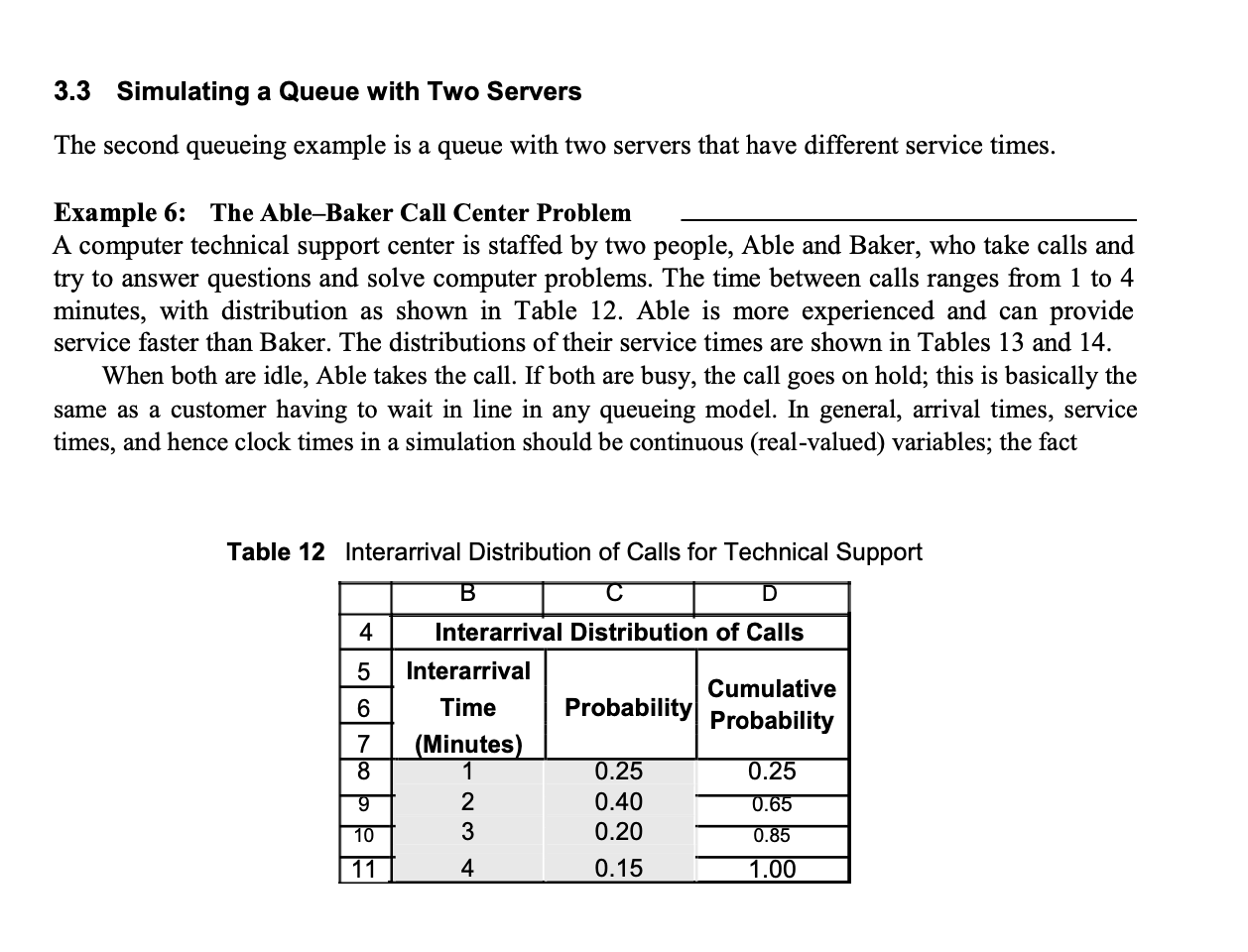
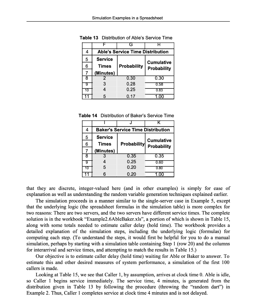
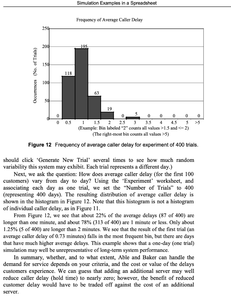
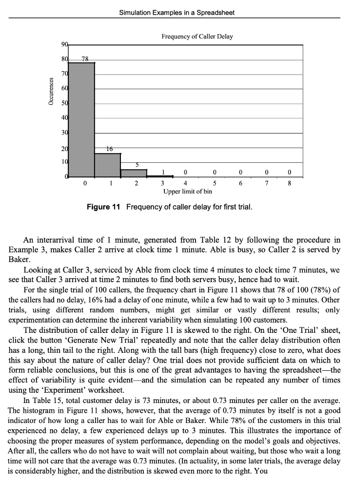
3.3 Simulating a Queue with Two Servers The second queueing example is a queue with two servers that have different service times. Example 6: The AbleBaker Call Center Problem A computer technical support center is staffed by two people, Able and Baker, who take calls and try to answer questions and solve computer problems. The time between calls ranges from 1 to 4 minutes, with distribution as shown in Table 12. Able is more experienced and can provide service faster than Baker. The distributions of their service times are shown in Tables 13 and 14. When both are idle, Able takes the call. If both are busy, the call goes on hold; this is basically the same as a customer having to wait in line in any queueing model. In general, arrival times, service times, and hence clock times in a simulation should be continuous (real-valued) variables; the fact Table 12 Interarrival Distribution of Calls for Technical Support B D 4 5 6 7 8 Interarrival Distribution of Calls Interarrival Cumulative Time Probability Probability (Minutes) 1 0.25 0.25 2 0.40 0.65 3 0.20 0.85 4 0.15 1.00 9 10 - WN 11 Simulation Examples in a Spreadsheet Table 13 Distribution of Able's Service Time F G 4 Able's Service Time Distribution 5 Service Cumulative 6 Times Probability Probability 7 (Minutes) 8 2 0.30 0.30 9 3 0.28 10 4 0.25 0.83 11 5 0.17 1.00 0.58 Table 14 Distribution of Baker's Service Time J 4 Baker's Service Time Distribution 5 Service Cumulative 6 Times 7 (Minutes) 8 3 0.35 0.35 9 4 0.25 0.60 10 5 0.20 0.80 11 6 0.20 1.00 Probability Probability that they are discrete, integer-valued here (and in other examples) is simply for ease of explanation as well as understanding the random variable generation techniques explained earlier. The simulation proceeds in a manner similar to the single-server case in Example 5, except that the underlying logic (the spreadsheet formulas in the simulation table) is more complex for two reasons: There are two servers, and the two servers have different service times. The complete solution is in the workbook Example2.6AbleBaker.xls, a portion of which is shown in Table 15, along with some totals needed to estimate caller delay (hold time). The workbook provides a detailed explanation of the simulation steps, including the underlying logic (formulas) for computing each step. (To understand the steps, it would first be helpful for you to do a manual simulation, perhaps by starting with a simulation table containing Step 1 (row 20) and the columns for interarrival and service times, and attempting to match the results in Table 15.) Our objective is to estimate caller delay (hold time) waiting for Able or Baker to answer. To estimate this and other desired measures of system performance, a simulation of the first 100 callers is made. Looking at Table 15, we see that Caller 1, by assumption, arrives at clock time 0. Able is idle, so Caller 1 begins service immediately. The service time, 4 minutes, is generated from the distribution given in Table 13 by following the procedure (throwing the "random dart") in Example 2. Thus, Caller 1 completes service at clock time 4 minutes and is not delayed. Simulation Examples in a Spreadsheet Frequency of Average Caller Delay 250 200 195. 150 118 Occurrences (No. of Trials) 100 63 0 >5 0 19 0 5 0 0 0 0 1 1.5 2 2.5 3 3.5 4 4.5 5 (Example: Bin labeled "2" counts all values >1.5 and 5) 0.5 Figure 12 Frequency of average caller delay for experiment of 400 trials. should click 'Generate New Trial' several times to see how much random variability this system may exhibit. Each trial represents a different day.) Next, we ask the question: How does average caller delay (for the first 100 customers) vary from day to day? Using the Experiment worksheet, and associating each day as one trial, we set the "Number of Trials to 400 (representing 400 days). The resulting distribution of average caller delay is shown in the histogram in Figure 12. Note that this histogram is not a histogram of individual caller delay, as in Figure 11. From Figure 12, we see that about 22% of the average delays (87 of 400) are longer than one minute, and about 78% (313 of 400) are 1 minute or less. Only about 1.25% (5 of 400) are longer than 2 minutes. We see that the result of the first trial (an average caller delay of 0.73 minutes) falls in the most frequent bin, but there are days that have much higher average delays. This example shows that a one-day (one trial) simulation may well be unrepresentative of long-term system performance. In summary, whether, and to what extent, Able and Baker can handle the demand for service depends on your criteria, and the cost or value of the delays customers experience. We can guess that adding an additional server may well reduce caller delay (hold time) to nearly zero; however, the benefit of reduced customer delay would have to be traded off against the cost of an additional server. Simulation Examples in a Spreadsheet Frequency of Caller Delay 90 80 78 70 60 Occurrences 50 40 30 20 10 0 0 0 8 0 1 0 0 3 4 5 Upper limit of bin 2 6 7 Figure 11 Frequency of caller delay for first trial. An interarrival time of 1 minute, generated from Table 12 by following the procedure in Example 3, makes Caller 2 arrive at clock time 1 minute. Able is busy, so Caller 2 is served by Baker. Looking at Caller 3, serviced by Able from clock time 4 minutes to clock time 7 minutes, we see that Caller 3 arrived at time 2 minutes to find both servers busy, hence had to wait. For the single trial of 100 callers, the frequency chart in Figure 11 shows that 78 of 100 (78%) of the callers had no delay, 16% had a delay of one minute, while a few had to wait up to 3 minutes. Other trials, using different random numbers, might get similar or vastly different results; only experimentation can determine the inherent variability when simulating 100 customers. The distribution of caller delay in Figure 11 is skewed to the right. On the 'One Trial' sheet, click the button Generate New Trial repeatedly and note that the caller delay distribution often has a long, thin tail to the right. Along with the tall bars (high frequency) close to zero, what does this say about the nature of caller delay? One trial does not provide sufficient data on which to form reliable conclusions, but this is one of the great advantages to having the spreadsheetthe effect of variability is quite evident and the simulation can be repeated any number of times using the 'Experiment' worksheet. In Table 15, total customer delay is 73 minutes, or about 0.73 minutes per caller on the average. The histogram in Figure 11 shows, however, that the average of 0.73 minutes by itself is not a good indicator of how long a caller has to wait for Able or Baker. While 78% of the customers in this trial experienced no delay, a few experienced delays up to 3 minutes. This illustrates the importance of choosing the proper measures of system performance, depending the model's goals and objectives. After all, the callers who do not have to wait will not complain about waiting, but those who wait a long time will not care that the average was 0.73 minutes. (In actuality, in some later trials, the average delay is considerably higher, and the distribution is skewed even more to the right. You