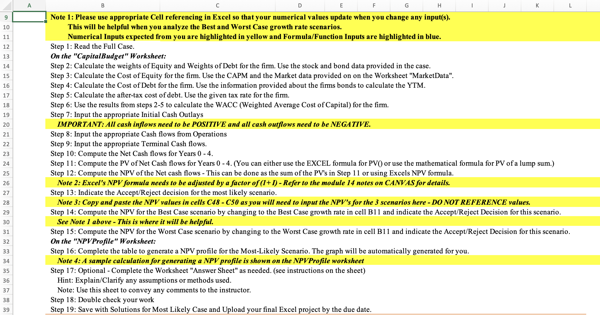
Note $1$: Please use appropriate Cell referencing in Excel so that your numerical values update when you change any input$($s$).$

This will be helpful when you analyze the Best and Worst Case growth rate scenarios.

Numerical Inputs expected from you are highlighted in yellow and Formula$/$Function Inputs are highlighted in blue.

Step $1$: Read the Full Case.

On the "CapitalBudget" Worksheet:

Step $2$: Calculate the weights of Equity and Weights of Debt for the firm. Use the stock and bond data provided in the case.

Step $3$: Calculate the Cost of Equity for the firm. Use the CAPM and the Market data provided on on the Worksheet "MarketData".

Step $4$: Calculate the Cost of Debt for the firm. Use the information provided about the firms bonds to calculate the YTM$.$

Step $5$: Calculate the after$-$tax cost of debt. Use the given tax rate for the firm.

Step $6$: Use the results from steps $2-5$ to calculate the WACC $($Weighted Average Cost of Capital$)$ for the firm.

Step $7$: Input the appropriate Initial Cash Outlays

IMPORTANT: All cash inflows need to be POSITIVE and all cash outflows need to be NEGATIVE.

Step $8$: Input the appropriate Cash flows from Operations

Step $9$: Input the appropriate Terminal Cash flows.

Step $10$: Compute the Net Cash flows for Years $0-4.$

Step $12$: Compute the NPV of the Net cash flows $-$ This can be done as the sum of the PV$\text{'}$s in Step $11$ or using Excels NPV formula.

Note $2$: Excel's NPV formula needs to be adjusted by a factor of $(1+I)-$Refer to the module $14$ notes on CANVAS for details.

Step $13$: Indicate the Accept$/$Reject decision for the most likely scenario.

Note $3$: Copy and paste the NPV values in cells C$48-$ C$50$ as you will need to input the NPV$\text{'}$s for the $3$ scenarios here $-$ DO NOT REFERENCE values.

See Note $1$ above $-$ This is where it will be helpful.

On the "NPVProfile" Worksheet:

Step $16$: Complete the table to generate a NPV profile for the Most$-$Likely Scenario. The graph will be automatically generated for you.

Note $4$: A sample calculation for generating a NPV profile is shown on the NPVProfile worksheet

Step $17$: Optional $-$ Complete the Worksheet "Answer Sheet" as needed. $($see instructions on the sheet$)$

Hint: Explain$/$Clarify any assumptions or methods used.

Note: Use this sheet to convey any comments to the instructor.

Step $18$: Double check your work

Step $19$: Save with Solutions for Most Likely Case and Upload your final Excel project by the due date.