(NOTE: I DO NOT NEED HELP WITH PROBLEM #'s 2-7, THEY ARE ONLY THERE FOR YOUR REFERENCE)

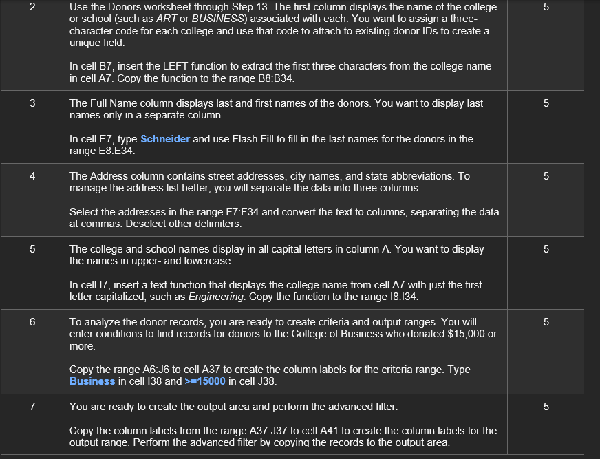
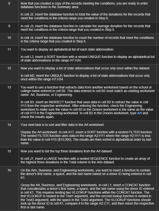
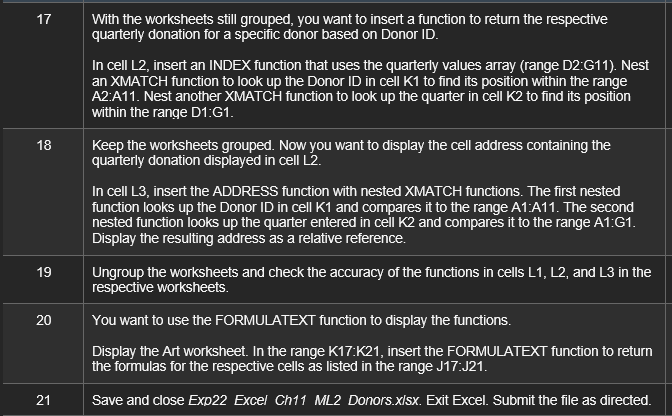
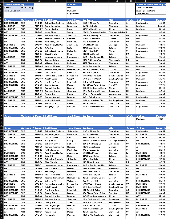
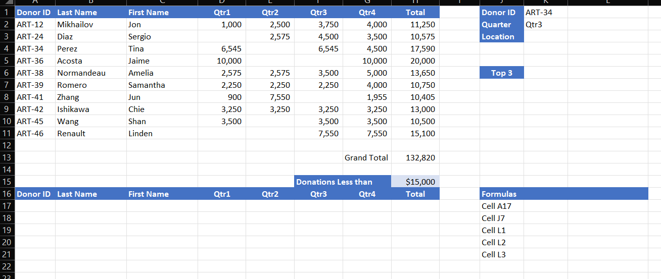
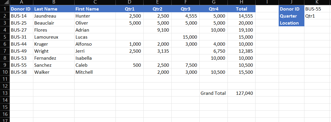
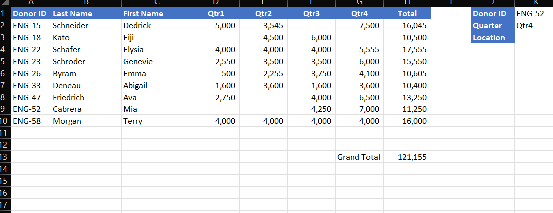
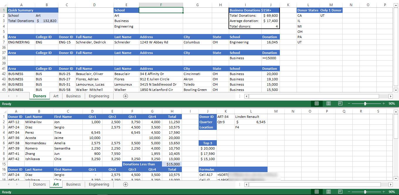
Use the Donors worksheet through Step 13. The first column displays the name of the college or school (such as ART or BUSINESS) associated with each. You want to assign a threecharacter code for each college and use that code to attach to existing donor IDs to create a unique field. In cell B7, insert the LEFT function to extract the first three characters from the college name in cell A7. Copy the function to the range B8:B34. The Full Name column displays last and first names of the donors. You want to display last names only in a separate column. In cell E7, type Schneider and use Flash Fill to fill in the last names for the donors in the range E8:E34 The Address column contains street addresses, city names, and state abbreviations. To manage the address list better, you will separate the data into three columns. Select the addresses in the range F7:F34 and convert the text to columns, separating the data at commas. Deselect other delimiters. The college and school names display in all capital letters in column A. You want to display the names in upper- and lowercase. In cell 17, insert a text function that displays the college name from cell A7 with just the first letter capitalized, such as Engineering. Copy the function to the range I8:I34. To analyze the donor records, you are ready to create criteria and output ranges. You will enter conditions to find records for donors to the College of Business who donated $15,000 or more. Copy the range A6:J6 to cell A37 to create the column labels for the criteria range. Type Business in cell I38 and >=15000 in cell J38. You are ready to create the output area and perform the advanced filter. Copy the column labels from the range A37:J37 to cell A41 to create the column labels for the output range. Perform the advanced filter by copying the records to the output area. 8 Now that you created a copy of the records meeting the conditions, you are ready to enter database functions in the Summary area. In cell J2, insert the database function to total the value of the donations for the records that meet the conditions in the criteria range you created in Step 6. In cell J3, insert the database function to calculate the average donation for the records that meet the conditions in the criteria range that you created in Step 6. In cell J4, insert the database function to count the number of records that meet the conditions in the criteria range that you created in Step 6. You want to display an alphabetical list of each state abbreviation. In cell L2, insert a SORT function with a nested UNIQUE function to display an alphabetical list of state abbreviations in the range H7:H34. Now you want to display a list of state abbreviations that occur only once within the dataset. In cell M2, insert the UNIQUE function to display a list of state abbreviations that occur only once within the range H7:H34. You want to use a function that extracts data from another worksheet based on the school or college name entered in cell B2. The data entered in cell B2 must match an existing worksheet name: Art, Business, or Engineering. In cell B3, insert an INDIRECT function that uses data in cell B2 to extract the value in cell H13 from the respective worksheet. After entering the function, check the Engineering worksheet to make sure the value in cell B3 in the Donors worksheet is the same as the value of cell H13 in the Engineering worksheet. In cell B2 in the Donors worksheet, type Art and check the results again. Your next task is to sort and filter data in the Art worksheet. Display the Art worksheet. In cell A17, insert a SORT function with a nested FILTER function. The nested FILTER function uses data in the range A2:H11 where the range H2 : H11 is less than the value in cell H15($15,000). The results are then sorted in alphabetical order by last name. Now you want to list the top three donations from the Art dataset. In cell J7, insert a LARGE function with a nested SEQUENCE function to create an array of the highest three donations in the Total column in the Arts dataset. On the Arts, Business, and Engineering worksheets, you want to insert a function to contain the donor's first name, a space, and the last name based on a donor ID being entered in cell K1. Group the Art, Business, and Engineering worksheets. In cell L1, insert a CONCAT function that concatenates a donor's first name, a space, and the last name using the donor ID entered in cell K1. This requires nesting two VLOOKUP functions within the CONCAT function. The first VLOOKUP is nested in the Text1 argument, and the second lookup function is nested in the Text3 argument, with the space in the Text2 argument. The VLOOKUP functions should look up the donor ID in cell K1, compare it to the range A2:C11, and then return the respective first or last name. 17 With the worksheets still grouped, you want to insert a function to return the respective quarterly donation for a specific donor based on Donor ID. In cell L2, insert an INDEX function that uses the quarterly values array (range D2:G11). Nest an XMATCH function to look up the Donor ID in cell K1 to find its position within the range A2:A11. Nest another XMATCH function to look up the quarter in cell K2 to find its position within the range D1:G1. 18 Keep the worksheets grouped. Now you want to display the cell address containing the quarterly donation displayed in cell L2. In cell L3, insert the ADDRESS function with nested XMATCH functions. The first nested function looks up the Donor ID in cell K1 and compares it to the range A1:A11. The second nested function looks up the quarter entered in cell K2 and compares it to the range A1:G1. Display the resulting address as a relative reference. 19 Ungroup the worksheets and check the accuracy of the functions in cells L1, L2, and L3 in the respective worksheets. 20 You want to use the FORMULATEXT function to display the functions. Display the Art worksheet. In the range K17:K21, insert the FORMULATEXT function to return the formulas for the respective cells as listed in the range J17:J21. 21 Save and close Exp22 Excel Ch11 ML2 Donors.xIsx. Exit Excel. Submit the file as directed. Grand Total 127,040 Grand Total 121,155 Use the Donors worksheet through Step 13. The first column displays the name of the college or school (such as ART or BUSINESS) associated with each. You want to assign a threecharacter code for each college and use that code to attach to existing donor IDs to create a unique field. In cell B7, insert the LEFT function to extract the first three characters from the college name in cell A7. Copy the function to the range B8:B34. The Full Name column displays last and first names of the donors. You want to display last names only in a separate column. In cell E7, type Schneider and use Flash Fill to fill in the last names for the donors in the range E8:E34 The Address column contains street addresses, city names, and state abbreviations. To manage the address list better, you will separate the data into three columns. Select the addresses in the range F7:F34 and convert the text to columns, separating the data at commas. Deselect other delimiters. The college and school names display in all capital letters in column A. You want to display the names in upper- and lowercase. In cell 17, insert a text function that displays the college name from cell A7 with just the first letter capitalized, such as Engineering. Copy the function to the range I8:I34. To analyze the donor records, you are ready to create criteria and output ranges. You will enter conditions to find records for donors to the College of Business who donated $15,000 or more. Copy the range A6:J6 to cell A37 to create the column labels for the criteria range. Type Business in cell I38 and >=15000 in cell J38. You are ready to create the output area and perform the advanced filter. Copy the column labels from the range A37:J37 to cell A41 to create the column labels for the output range. Perform the advanced filter by copying the records to the output area. 8 Now that you created a copy of the records meeting the conditions, you are ready to enter database functions in the Summary area. In cell J2, insert the database function to total the value of the donations for the records that meet the conditions in the criteria range you created in Step 6. In cell J3, insert the database function to calculate the average donation for the records that meet the conditions in the criteria range that you created in Step 6. In cell J4, insert the database function to count the number of records that meet the conditions in the criteria range that you created in Step 6. You want to display an alphabetical list of each state abbreviation. In cell L2, insert a SORT function with a nested UNIQUE function to display an alphabetical list of state abbreviations in the range H7:H34. Now you want to display a list of state abbreviations that occur only once within the dataset. In cell M2, insert the UNIQUE function to display a list of state abbreviations that occur only once within the range H7:H34. You want to use a function that extracts data from another worksheet based on the school or college name entered in cell B2. The data entered in cell B2 must match an existing worksheet name: Art, Business, or Engineering. In cell B3, insert an INDIRECT function that uses data in cell B2 to extract the value in cell H13 from the respective worksheet. After entering the function, check the Engineering worksheet to make sure the value in cell B3 in the Donors worksheet is the same as the value of cell H13 in the Engineering worksheet. In cell B2 in the Donors worksheet, type Art and check the results again. Your next task is to sort and filter data in the Art worksheet. Display the Art worksheet. In cell A17, insert a SORT function with a nested FILTER function. The nested FILTER function uses data in the range A2:H11 where the range H2 : H11 is less than the value in cell H15($15,000). The results are then sorted in alphabetical order by last name. Now you want to list the top three donations from the Art dataset. In cell J7, insert a LARGE function with a nested SEQUENCE function to create an array of the highest three donations in the Total column in the Arts dataset. On the Arts, Business, and Engineering worksheets, you want to insert a function to contain the donor's first name, a space, and the last name based on a donor ID being entered in cell K1. Group the Art, Business, and Engineering worksheets. In cell L1, insert a CONCAT function that concatenates a donor's first name, a space, and the last name using the donor ID entered in cell K1. This requires nesting two VLOOKUP functions within the CONCAT function. The first VLOOKUP is nested in the Text1 argument, and the second lookup function is nested in the Text3 argument, with the space in the Text2 argument. The VLOOKUP functions should look up the donor ID in cell K1, compare it to the range A2:C11, and then return the respective first or last name. 17 With the worksheets still grouped, you want to insert a function to return the respective quarterly donation for a specific donor based on Donor ID. In cell L2, insert an INDEX function that uses the quarterly values array (range D2:G11). Nest an XMATCH function to look up the Donor ID in cell K1 to find its position within the range A2:A11. Nest another XMATCH function to look up the quarter in cell K2 to find its position within the range D1:G1. 18 Keep the worksheets grouped. Now you want to display the cell address containing the quarterly donation displayed in cell L2. In cell L3, insert the ADDRESS function with nested XMATCH functions. The first nested function looks up the Donor ID in cell K1 and compares it to the range A1:A11. The second nested function looks up the quarter entered in cell K2 and compares it to the range A1:G1. Display the resulting address as a relative reference. 19 Ungroup the worksheets and check the accuracy of the functions in cells L1, L2, and L3 in the respective worksheets. 20 You want to use the FORMULATEXT function to display the functions. Display the Art worksheet. In the range K17:K21, insert the FORMULATEXT function to return the formulas for the respective cells as listed in the range J17:J21. 21 Save and close Exp22 Excel Ch11 ML2 Donors.xIsx. Exit Excel. Submit the file as directed. Grand Total 127,040 Grand Total 121,155