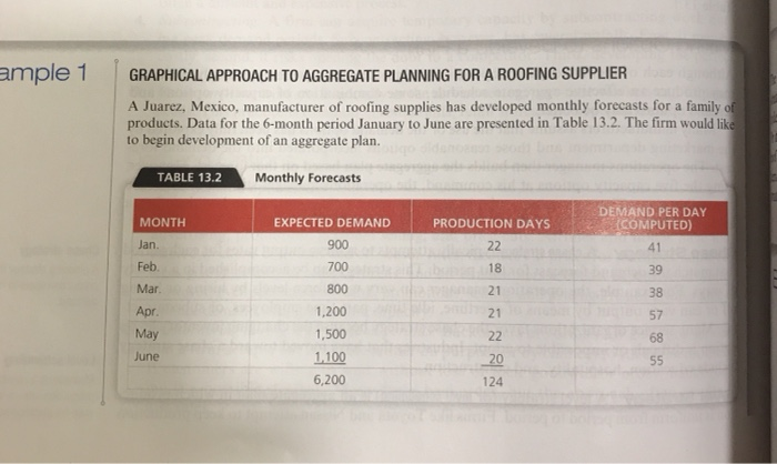
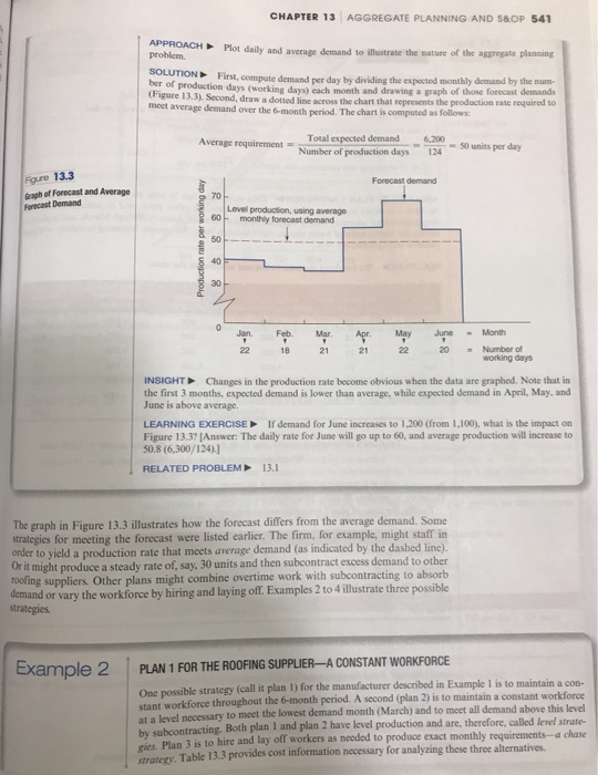
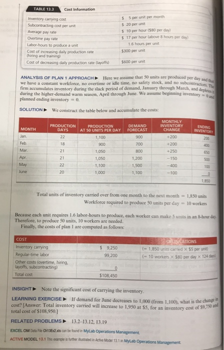
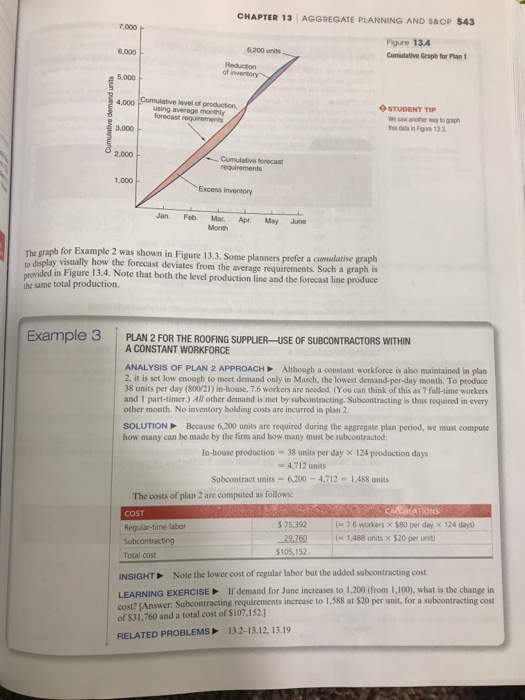
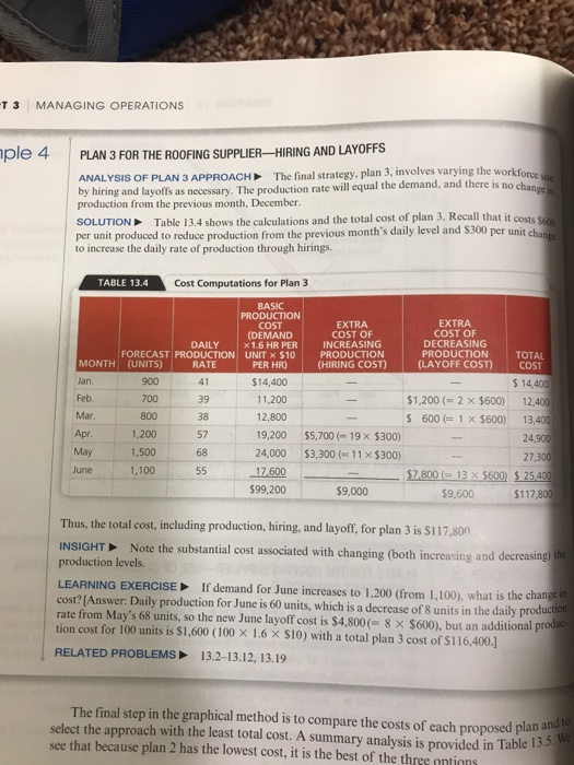
Operations Management II Chapter 13 Aggregate Planning 1. For the roofing manufacturer described in Examples 1 to 4 of this chapter, evaluate the cost for the 6 month period for the following plans: (Use the information found in Table 13.3 also assume inventory starts at zero but might not end at zero for each plan) A. Maintain a constant work force required in Jan use overtime pay when required to meet demand. B. Maintain a constant work force required in Jan use subcontractors when required to meet demand. C. Maintain a constant work force required in Jan. Hire and layoff workers as required each month to meet demand. ample 1 GRAPHICAL APPROACH TO AGGREGATE PLANNING FOR A ROOFING SUPPLIER A Juarez, Mexico, manufacturer of roofing supplies has developed monthly forecasts for a family of products. Data for the 6-month period January to June are presented in Table 13.2. The firm would like to begin development of an aggregate plan. TABLE 13.2 Monthly Forecasts MONTH PRODUCTION DAYS DEMAND PER DAY COMPUTED) Jan. EXPECTED DEMAND 900 700 22 41 Feb. 18 39 Mar. 800 21 38 21 57 Apr. May June 22 68 1,200 1,500 1,100 6,200 20 55 124 CHAPTER 13 AGGREGATE PLANNING AND S&OP 541 APPROACH Plot daily and average demand to illustrate the nature of the aggregate planning problem SOLUTION First compute demand per day by dividing the expected monthly demand by the num ber of production days (working days) each month and drawing a graph of those forecast demands (Figure 13.3). Second, draw a dotted line across the chart that represents the production rate required to meet average demand over the 6-month period. The chart is computed as follows: Average requirement Total expected demand Number of production days 6.200 124 - 50 units per day Foure 13.3 Forecast demand Graph of Forecast and Average Forecast Demand 70 60 Level production, using average monthly forecast demand Production rate per working day 50 40 30 0 Jan. Feb Mar June May 1 22 22 18 21 21 20 Month - Number of working days INSIGHT Changes in the production rate become obvious when the data are graphed. Note that in the first 3 months, expected demand is lower than average, while expected demand in April, May, and June is above average LEARNING EXERCISE If demand for June increases to 1,200 (from 1.100), what is the impact on Figure 13.3? (Answer: The daily rate for June will go up to 60, and average production will increase to 50.8 (6,300/124).] RELATED PROBLEM 13.1 The graph in Figure 13.3 illustrates how the forecast differs from the average demand. Some strategies for meeting the forecast were listed earlier. The firm, for example, might staff in order to yield a production rate that meets average demand (as indicated by the dashed line). Or it might produce a steady rate of, say, 30 units and then subcontract excess demand to other roofing suppliers Other plans might combine overtime work with subcontracting to absorb demand or vary the workforce by hiring and laying off. Examples 2 to 4 illustrate three possible strategies Example 2 PLAN 1 FOR THE ROOFING SUPPLIER-A CONSTANT WORKFORCE One possible strategy (call it plan 1) for the manufacturer described in Example 1 is to maintain a con- stant workforce throughout the 6-month period. A second (plan 2) is to maintain a constant workforce at a level necessary to meet the lowest dem month (March) and to meet all demand above this level by subcontracting. Both plan 1 and plan 2 have level production and are, therefore, called level strate- gies. Plan 3 is to hire and lay off workers as needed to produce exact monthly requirements-a chase strategy. Table 13.3 provides cost information necessary for analyzing these three alternatives. we have a constant workforce, no overtime or idle time, no safety stock, and to subcontractors. The TABLE 13.3 Cost Information Inventory Carrying cost Subcontracting cost per unit Average pay rate Overtime pay rate Labor hours to produce a unit Cost of increasing daily production rate Chiring and training) Cost of decreasing daily production rate (layoffs) $5 per unit per month $ 20 per unit $10 per hour (580 per day $17 per hour above 8 hours per day 1.6 hours per unit $300 per unit 5600 per unit ANALYSIS OF PLAN 1 APPROACH Here we assume that 50 units are produced per day and the firm accumulates inventory during the slack period of demand, January through March, and depletes during the higher-demand warm season, April through June. We assume beginning inventory and planned ending inventory = 0. SOLUTION We construct the table below and accumulate the costs: PRODUCTION AT SO UNITS PER DAY DEMAND FORECAST ENDING INVENTORY 200 1.100 900 100 MONTH Jan Feb Mar Apr. May June PRODUCTION DAYS 22 18 21 21 22 20 700 800 900 1,050 1,050 1.100 1,000 MONTHLY INVENTORY CHANGE -200 -200 +250 - 150 -400 -100 550 500 1.200 1,500 1,100 100 1,850 Total units of inventory carried over from one month to the next month = 1,850 units Workforce required to produce 50 units per day - 10 workers Because each unit requires 16 labor-hours to produce, each worker can make 3 units in an 8-hour day Therefore, to produce 50 units, 10 workers are needed. Finally, the costs of plan I are computed as follows: COST Inventory carrying Regular-time labor Other costs (overtime, hiring, layoffs, subcontracting) Total cost $ 9.250 99,200 EATIONS (= 1,850 units carried x 55 per unit (-10 workers x 580 per day x 124 $108,450 INSIGHT Note the significant cost of carrying the inventory. LEARNING EXERCISE If demand for June decreases to 1.000 (from 1.100), what is the change in cost? (Answer: Total inventory carried will increase to 1,950 at SS, for an inventory cost of 59,750 and total cost of $108,950. RELATED PROBLEMS 13.2-13.12, 13.19 EXCEL OM Duta Fe Ch1352xls can be found in MyLab Operations Management ACTIVE MODEL 18.1 This ample is further llustrated in Active Model 13.1 in Mylab Operations Management CHAPTER 13 AGGREGATE PLANNING AND S&OP 543 7.000 6,000 6,200 units Figure 13.4 Cumulative Graph for Plant Reduction of inventory 5,000 4.000 Cumulative level of production using average monthly forecast requirements 3,000 STUDENT TIP Cumulative demand units this data in gure 133 2.000 Cumulative forecast requirements 1.000 Excess inventory Jan Feb Mar Month Apr May June The graph for Example 2 was shown in Figure 13.3. Some planners prefer a cumulative graph no display visually how the forecast deviates from the average requirements. Such a graph is provided in Figure 13.4. Note that both the level production line and the forecast line produce the same total production. Example 3 PLAN 2 FOR THE ROOFING SUPPLIER-USE OF SUBCONTRACTORS WITHIN A CONSTANT WORKFORCE ANALYSIS OF PLAN 2 APPROACH Although a constant workforce is also maintained in plan 2. it is set low enough to meet demand only in March, the lowest demand-per-day month. To produce 38 units per day (800/21) in-house, 7.6 workers are needed. (You can think of this as 7 full-time workers and 1 part-timer. All other demand is met by subcontracting. Subcontracting is thus required in every other month. No inventory holding costs are incurred in plan 2. SOLUTION Because 6.200 units are required during the aggregate plan period, we must compute how many can be made by the firm and how many lust be subcontracted: In-house production - 38 units per day X 124 production days = 4.712 units Subcontract units - 6,200 - 4,712 - 1.488 units The costs of plan 2 are computed as follows CACATIONS $ 75,392 (= 7.6 workers x 580 per day x 124 days) 29,760 Subcontracting (-1,488 units x 520 per unit) $105,152 Total cost COST Regular-time labor INSIGHT Note the lower cost of regular labor but the added subcontracting cost, LEARNING EXERCISE If demand for June increases to 1,200 (from 1,100), what is the change in cost? [Answer: Subcontracting requirements increase to 1,588 at $20 per unit, for a subcontracting cost of $31.760 and a total cost of S107.152.] RELATED PROBLEMS 13.2-13.12, 13.19 T 3 MANAGING OPERATIONS ople 4 PLAN 3 FOR THE ROOFING SUPPLIER-HIRING AND LAYOFFS ANALYSIS OF PLAN 3 APPROACH The final strategy, plan 3, involves varying the workforce by hiring and layoffs as necessary. The production rate will equal the demand, and there is no change in production from the previous month, December SOLUTION Table 13.4 shows the calculations and the total cost of plan 3. Recall that it costs 5600 per unit produced to reduce production from the previous month's daily level and S300 per unit change to increase the daily rate of production through hirings. COST TABLE 13.4 Cost Computations for Plan 3 BASIC PRODUCTION COST EXTRA EXTRA (DEMAND COST OF COST OF DAILY x1.6 HR PER INCREASING DECREASING FORECAST PRODUCTION UNIT X 510 PRODUCTION PRODUCTION TOTAL MONTH (UNITS) RATE PER HR) (HIRING COST) (LAYOFF COST) Jan 900 41 $14,400 $ 14,400 Feb. 700 39 11,200 $1,200 (= 2 x 5600) 12,400 Mar 800 38 12,800 $ 600 = 1 X 5600) 13,400 Apr. 1,200 57 19,200 55,700 (-19 x 5300) 24.900 1,500 68 24,000 $3,300 (-11 X $300) 27,300 June 1,100 55 17,600 $7 800 = 13 x 5600) $ 25.400 $99,200 $9.000 $9,600 $117,800 May Thus, the total cost, including production, hiring, and layoff, for plan 3 is $117,800 INSIGHT Note the substantial cost associated with changing (both increasing and decreasing the production levels. LEARNING EXERCISE If demand for June increases to 1,200 (from 1,100), what is the change in cost? Answer: Daily production for June is 60 units, which is a decrease of 8 units in the daily production rate from May's 68 units, so the new June layoff cost is $4,800(= 8 x $600), but an additional produc tion cost for 100 units is $1,600 (100 X 1.6 X S10) with a total plan 3 cost of $116,400.] RELATED PROBLEMS 13.2-13.12, 13.19 The final step in the graphical method is to compare the costs of each proposed plan and te select the approach with the least total cost. A summary analysis is provided in Table 13.5. We see that because plan 2 has the lowest cost, it is the best of the three antions